Causal Fair Machine Learning Methods
Most recent fairness notions are causality-based and reflect the now widely accepted idea that using causality is necessary to appropriately address the problem of fairness. Causality-based fairness notions differ from the statistical ones in that they are not totally based on data, but consider additional knowledge about the structure of the world, in the form of a causal model.
Causality-based fairness notions are developed mainly under two causal frameworks: the structural causal model (SCMs) and the potential outcome. SCMs assume that we know the complete causal graph, and hence, we are able to study the causal effect of any variable along many different paths. The potential outcome framework does not assume the availability of the causal graph and instead focuses on estimating the causal effects of treatment variables. In the table below I present the causal framework to which each causality-based fairness notion discussed in this section belongs. In this section, we we begin by giving a short insight and overview of causality-based fairness notions, followed by a brief intermission to introduce two important statistical-fairness definitions, and then we spend the remainder of the section introducing the casual-based fairness notions, minus the last section where we state the main technical pitfalls experienced by these types of metrics.
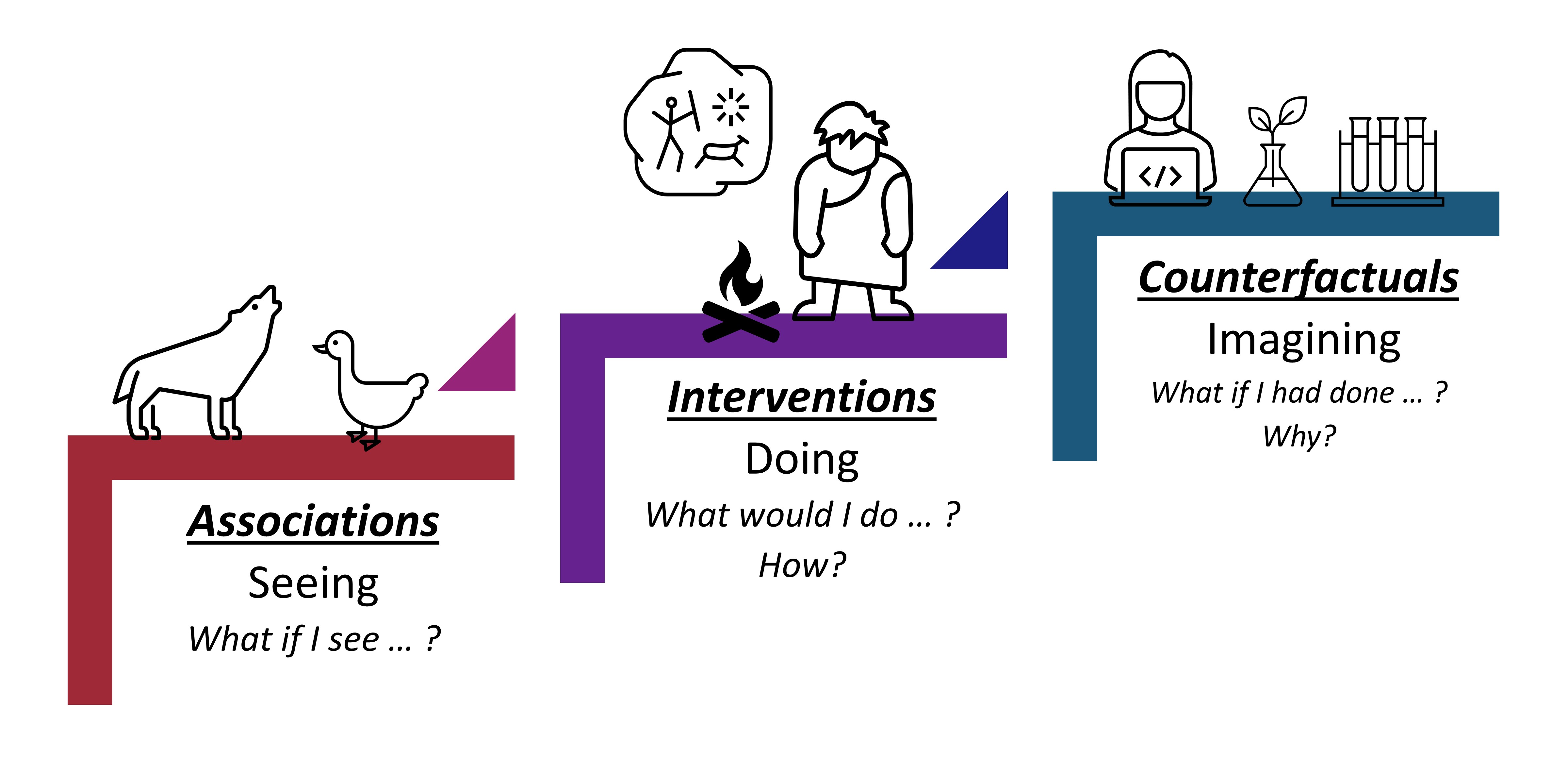
In [1], Pearl presented the causal hierarchy through the Ladder of Causation, as shown in the figure above. The Ladder of Causation has the 3 rungs: association, intervention, and counterfactual. The first rung, associations, can be inferred directly from the observed data using conditional probabilities and conditional expectations. The intervention rung involves not only seeing what is, but also changing what we see. Interventional questions deal with $P(y\mid do(x), z)$ which stands for “the probability of $Y=y$, given that we intervene and set the values of $X$ to $x$ and subsequently observe event $Z=z$ .” Interventional questions cannot be answered from pure observational data alone. They can be estimated experimentally from randomized trials or analytically using causal Bayesian networks. The top rung invokes counterfactuals and deals with $P(y_x\mid x’, y’)$ which stands for “the probability that event $Y=y$ would be observed had $X$ been $x$, given that we actually observed $X$ to be $x’$ and $Y$ to be $y’$ .” Such questions can be computed only when the model is based on functional relations or is structural. In in the table below also show the causal hierarchical level that each causality-based fairness notion aligns with.
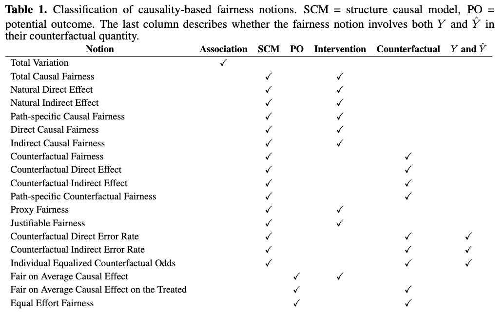
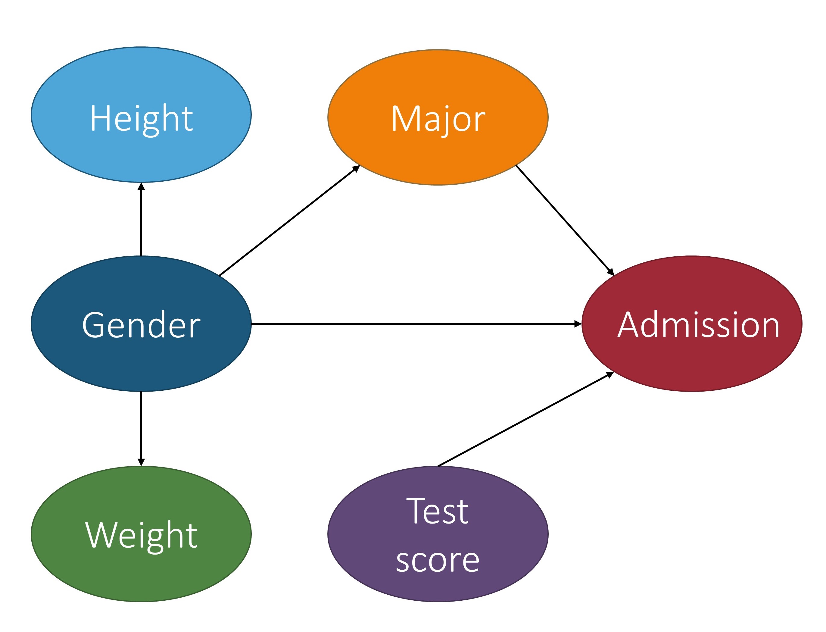
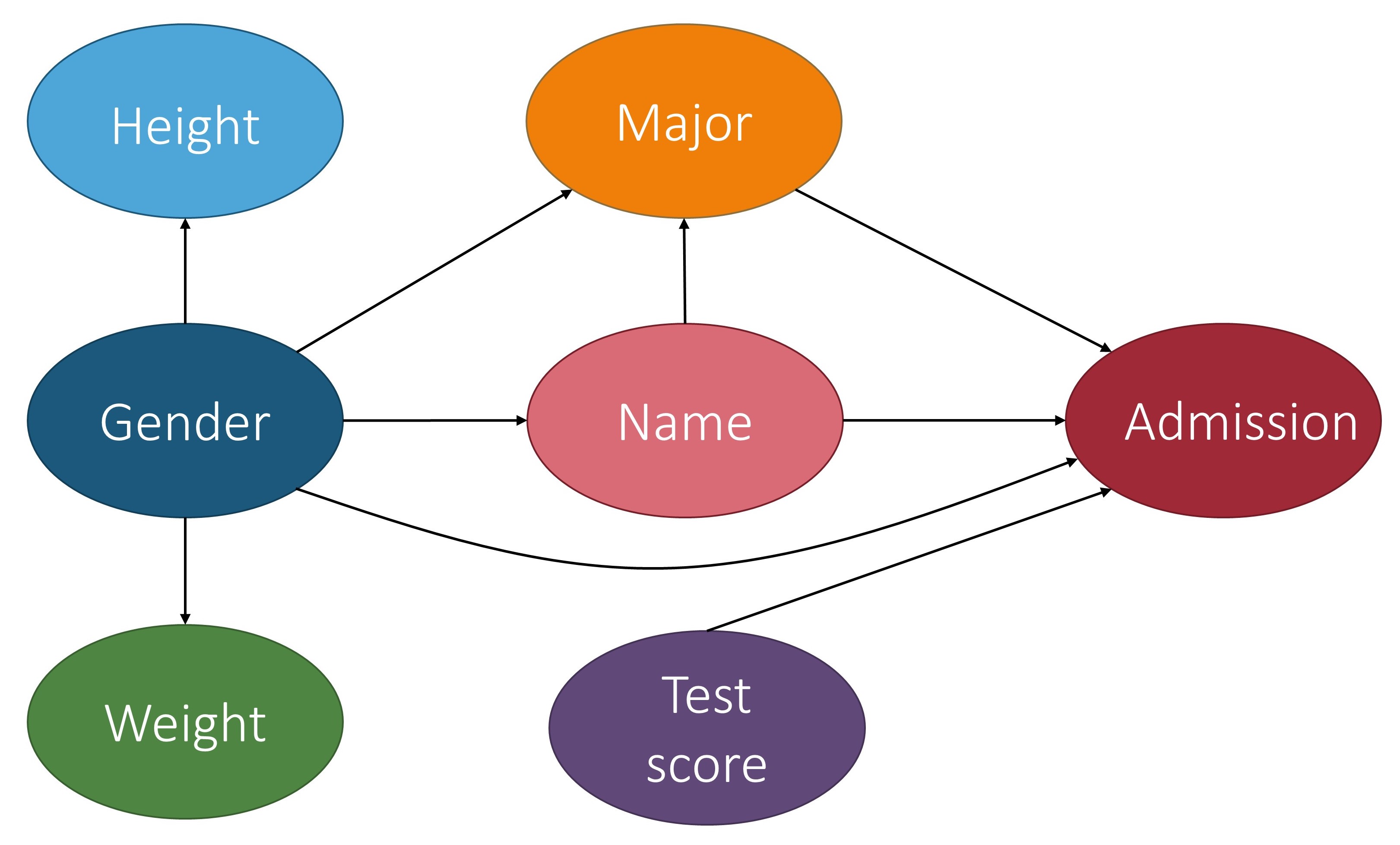
In the context of fair machine learning, we use $S \in {s^+, s^-}$ to denote the marginalization attribute, $Y \in {y^+, y^-}$ to denote the decision, and $\mathbf{X}$ to denote a set of non-marginalization attributes. The underlying mechanism of the population over the space $S\times \mathbf{X} \times Y$ is represented by a causal model $\mathcal{M}$, which is associated with a causal graph $\mathcal{G}$. The figure below shows a causal graph that will be used to illustrate fairness notions throughout this section. With $\mathcal{M}$, we want to reason about counterfactual queries, e.g., “what would the prediction have been for this individual if their marginalization attribute value changed?’’ A historical dataset $\mathcal{D}$ is drawn from the population, which is used to construct a predictor $ h: \mathbf{X}, S \rightarrow \hat{Y} $. Note that the input of the predictor can be a subset of $\mathbf{X}, S$ and we use $\widehat{Pa{}}$ to denote the set of input features of the predictor when introducing counterfactual error rate in Section \ref{sec:cer}. The causal model for the population over space $S\times \mathbf{X} \times \hat{Y}$ can be considered the same as $\mathcal{M}$, except that the function $f_{Y}$ is replaced with a predictor $h$. Most fairness notions involve either $Y$ or $\hat{Y}$ in their counterfactual quantity and, roughly speaking, they correspond to statistical parity (a statistical-based notion introduced below). A few fairness notions, e.g., counterfactual direct error rate [2], correspond to the concept of equalized odds (also explained below) and involve both $Y$ and $\hat{Y}$ in their counterfactual quantity. We also mark if a notion uses $Y$ and/or $\hat{Y}$ in the table abovoe.
We note that for all of the fairness notions presented here, there actually exists two versions – strict and relaxed. The strict version means there is absolutely no discrimination effect (i.e., no wiggle room), whereas the relaxed version often compares the causal effect with $\tau$, a user-defined threshold for discrimination (i.e., wiggle room). Despite having two approaches, for simplicity, we adhere to the strict version when introducing each fairness notion in the discussion below.
Total, Natural Direct, and Natural Indirect Causal Fairness
We now move into our main discussion of the causality-based fairness notions, starting with a discussion of total, natural direct, and natural indirect causal fairness. Discrimination can be viewed as the causal effect of $S$ on $Y$. Total causal fairness answers the question of if the marginalization attribute $S$ changed (e.g., changing from marginalized group $s^{-}$ to non-marginalized group $s^{+}$ ), how would the outcome $Y$ change on average? A straightforward strategy to answer this question is to measure the average causal effect of $S$ on $Y$ when $S$ changes from $s^{-}$ to $s^{+}$, an approach called total causal fairness.
 Definition: Total Causal Fairness
Given the marginalization attribute $S$ and decision $Y$, we achieve total causal fairness if:
$TCE(s_1, s_0) = P(y_{s_1}) - P(y_{s_0}) = 0$
where $s_1, s_0 \in { s^+, s^-}$.
For instance, based on the figure above, TCE would report the average causal effect that being Female had on a student’s outcome of admission.
Additionally, the causal effect of $S$ on $Y$ does not only include the direct discriminatory effect, but it also includes the indirect discriminatory effect and the explainable effect. In [3], Pearl proposed the use of NDE and NIE to measure the direct and indirect discrimination. Recall that $NDE(s_1, s_0) = P(y_{s_1, Z_{s_0}}) - P(y_{s_0})$ and $NIE(s_1, s_0) = P(y_{s_0, Z_{s_1}}) - P(y_{s_0})$ where $\mathbf{Z}$ is the set of mediator variables. When applied to the example above, the mediator variable could be the major.
$P(y_{s_1, Z_{s_0}})$ in NDE is the probability of $Y=y$ had $S$ been $s_1$ and had $\mathbf{Z}$ been the value it would naturally take if $S=s_0$ . In other words, based on the example, $P(y_{s_1, Z_{s_0}})$ would be the probability of being admitted when changing the gender to be Male while keeping the major the same. Similarly, NIE measures the indirect effect of $S$ on $Y$. However, NIE does not distinguish between explainable and indirect discrimination.
Path-Specific Causal Fairness
In [4], Zhang et al. introduced path-specific causal fairness based on path-specific causal effect [5]. Different from total, natural direct, and natural indirect causal effects, the path-specific causal effect is based on graph properties of the causal graph (where the others were based on probabilities), and characterizes the causal effect in term of specific paths.
Definition: Path-Specific Causal Fairness
Given the marginalization attribute $S$, decision $Y$, and redlining attributes $\mathbf{R}$ (i.e., a set of attributes in $\mathbf{X}$ that cannot be legally justified if used in decision-making), define $\pi_{d}$ as the path set that contains some paths from $S$ to $Y$. We achieve path-specific causal fairness if:
$PE_{\pi}(s_1,s_0) = P(y_{s_1 \vert \pi, s_0 \vert \overline{\pi}}) - P(s_{x_0}) =0$
where $s_1, s_0 \in { s^+, s^-}$. Specifically, define $\pi_{d}$ as the path set that contains only $S\rightarrow Y$ and define $\pi_{i}$ as the path set that contains all the causal paths from $S$ to $Y$ which pass through some redlining attributes of $\mathbf{R}$. We achieve direct causal fairness if $PE_{\pi_{d}}(s_1,s_0)=0$, and indirect causal fairness if $PE_{\pi_{i}}(s_1,s_0)=0$.
Direct discrimination considers the causal effect transmitted along the direct path from $S$ to $Y$, i.e., $S\rightarrow Y$. The physical meaning of $PE_{\pi_{d}}(s_1,s_0)$ can be explained as the expected change in decisions of individuals from marginalized group $s_0$, if the decision makers are told that these individuals were from the non-marginalized group $s_1$. When applied to the running example, it means that the expected change in admission of applicants is actually from the marginalized group (e.g., Female), when the admission office is instructed to treat the applicants as from the non-marginalized group (e.g., Male).
Indirect discrimination considers the causal effect transmitted along all the indirect paths from $S$ to $Y$ that contain the redlining attributes. The physical meaning of $PE_{\pi_{i}}(s_1,s_0)$ is the expected change in decisions of individuals from marginalized group $s_0$, if the values of the redlining attributes in the profiles of these individuals were changed as if they were from the non-marginalized group $s_1$. When applied to the example, it means the expected change in admission of the marginalized group if they had the same gender makeups shown in the major as the non-marginalized group.
The following propositions [4] further show two properties of the path-specific effect metrics.
Proposition
If path set $\pi$ contains all causal paths from $S$ to $Y$ and $S$ has no parent in $\mathcal{G}$, then we have:
$PE_{\pi}(s_1,s_0) = TCE(s_1,s_0) = P(y^{+}\mid s_1)-P(y^{+}\mid s_0)$
$P(y^{+}\mid s_1)-P(y^{+}\mid s_0)$ is known as the risk difference (a measure of statistical parity). Therefore, the path-specific effect metrics can be considered as an extension to the risk difference (and statistical parity) for explicitly distinguishing the discriminatory effects of direct and indirect discrimination from the total causal effect.
Proposition
For any path sets $\pi_{d}$ and $\pi_{i}$, we do not necessarily have:
$PE_{\pi_{d}}(s_1,s_0)+PE_{\pi_{i}}(s_1,s_0)=PE_{\pi_{d}\cup \pi_{i}}(s_1,s_0)$
This implies that there might not be a linear connection between direct and indirect discrimination.
Counterfactual Fairness
In counterfactual fairness and path-specific causal fairness, the intervention is performed on the whole population. These metrics deal with effects on an entire population, or on the average individual from a population. But, up to this point we have not talked about “personalized causation” – or causation at the level of particular events of individuals [6]. Counterfactuals will allow us to do so. If we infer the post-intervention distribution while conditioning on certain individuals, or groups specified by a subset of observed variables, the inferred quantity will involve two worlds simultaneously: the real world represented by causal model $\mathcal{M},$ as well as the counterfactual world $M_x$. Such causal inference problems are called counterfactual inference, and the distribution of $Y_{x}$ conditioning on the real world observation $\mathbf{O}=\mathbf{o}$ is denoted by $P(y_{x}\mid \mathbf{o})$.
In [7], Kusner et al. defined counterfactual fairness to be the case where the outcome would have remained the same had the marginalization attribute of an individual or a group been different, and all other attributes been equal.
Definition: Counterfactual Fairness
Given a factual condition $\mathbf{O}= \mathbf{o}$ where $\mathbf{O} \subseteq {S, \mathbf{X}, Y }$, we achieve counterfactual fairness if:
$CE(s_1, s_0\mid \mathbf{o}) = P(y_{s_1} \mid \mathbf{o}) - P(y_{s_0} \mid \mathbf{o}) =0$
where $s_1, s_0 \in { s^+, s^-}$ .
Counterfactual Effects
In [8], Zhang and Bareinboim introduced three fine-grained measures of the transmission of change from stimulus to effect called the counterfactual direct, indirect, and spurious effects. Throughout this section, we use $\mathbf{W}$ to denote all the observed intermediate variables between $S$ and $Y$ and use the group with $S=s_0$ as the baseline to measure changes of the outcome.
Definition: Counterfactual Direct Effect
Given a SCM, the counterfactual direct effect (Ctf-DE) of intervention $S=s_1$ on $Y$ (with baseline $s_0$) conditioned on $S=s$ is defined as:
$Ctf-DE_{s_0,s_1}(y\mid s) = P(y_{s_1,\mathbf{W_{s_0}}}\mid s) - P(y_{s_0}\mid s)$
$Y_{s_1,\mathbf{W}\(_{s_0}} = y\mid S = s$ is a more involved counterfactual compared to NDE and can be read as "the value $Y$ would be had $S$ been $s_1$, while $\mathbf{W}$ is kept at the same value that it would have attained had $S$ been $s_0$, given that $S$ was actually equal to $s$." In terms of the above figure, $Y_{s_1,\mathbf{W}\)_{s_0}} = y\mid S = s$ means the admission decision for a Female student if they had actually been Male, while keeping all intermediate variables the same, when given that the student’s gender is actually $s$ (meaning Male or Female).
Definition: Counterfactual Indirect Effect
Given a SCM, the counterfactual indirect effect (Ctf-IE) of intervention $S=s_1$ on $Y$ (with baseline $s_0$) conditioned on $S=s$ is defined as:
$Ctf-IE_{s_0,s_1}(y\mid s) = P(y_{s_0, W_{s_1}}\mid s) - P(y_{s_0}\mid s)$
Ctf-IE measures changes in the probability of the outcome $Y$ being $y$ had $S$ been $s_0$, while changing $\mathbf{W}$ to whatever level it would have naturally obtained had $S$ been $s_1$, in particular, for the individuals in which $S=s_0$. In terms of the example, this means the probability of admission for a Female student based on the intermediate variable values that would be obtained if they were Male (e.g., ratio of Males applying to the major).
Definition: Counterfactual Spurious Effect
Given a SCM, the counterfactual spurious effect (Ctf-SE) of $S=s_1$ on $Y=y$ (with baseline $s_0$) is defined as:
$Ctf-SE_{s_0,s_1}(y) = P(y_{s_0}\mid s_1) - P(y\mid {s_0})$
$Ctf-SE_{s_0,s_1}(y)$ measures the difference in the outcome $Y=y$ had $S$ been $s_0$ for the individuals that would naturally choose $S$ to be $s_0$ versus $s_1$. In other words, it measures the difference in the admission decision had the marginalization attribute been set to Female for the students that were actually Female versus Male.
Proposition
For a SCM, if $S$ has no direct (indirect) causal path connecting $Y$ in the causal graph, then $Ctf-DE_{s_0,s_1}(y\mid s)=0$ ($Ctf-IE_{s_0,s_1}(y\mid s)=0$) for any $s$, $y$; if $S$ has no back-door\footnote{A backdoor path from $X$ to $Y$ is any path starting at $X$ with a backward edge $\leftarrow$ into $X$ such as: $X \leftarrow A \rightarrow B \leftarrow C \rightarrow Y$. Backdoor paths allow information to flow from $X$ to $Y$ in a way that is not causal.} path connecting $Y$ in the causal graph, then $Ctf-SE_{s_0,s_1}(y) = 0$ for any $y$.
Building on these measures, Zhang and Bareinboim derived the causal explanation formula for the disparities observed in the total variation. Recall that the total variation is simply the difference between the conditional distributions of $Y$ when observing $S$ changing from $s_0$ to $s_1$.
Definition: Total Variation
The total variation (TV) of $S=s_1$ on $Y=y$ (with baseline $s_0$) is given by:
$TV_{s_0, s_1}(y) = P(y\mid s_1) - P(y\mid s_0)$
In regard to the figure above, the TV would be the probability of the outcome given that the student was Male minus the probability of the outcome given that the student was Female., i.e., the difference in their overall probabilites of being admitted.
*Theorem: Causal Explanation Formula**
For any $s_0$, $s_1$, $y$, the total variation, counterfactual spurious, direct, and indirect effects obey the following relationship:
$TV_{s_0,s_1}(y) = Ctf-SE_{s_0,s_1}(y) + Ctf-IE_{s_0,s_1}(y\mid s_1) - Ctf-DE_{s_1,s_0}(y\mid s_1)$
$TV_{s_0,s_1}(y) = Ctf-DE_{s_0,s_1}(y\mid s_0) - Ctf-SE_{s_1,s_0}(y) - Ctf-IE_{s_1,s_0}(y\mid s_0)$
The theorem allows the machine learning designer to quantitatively evaluate fairness and explain the total observed disparity of a decision through different discriminatory mechanisms. For example, the first formula shows that the total disparity experienced by the individuals who have naturally attained $s_1$ (relative to $s_0$, in other words, students who were naturally Male over Female) is equal to the disparity associated with spurious discrimination, plus the advantage it lost due to indirect discrimination, minus the advantage it would have gained without direct discrimination.
Path-Specific Counterfactual Fairness
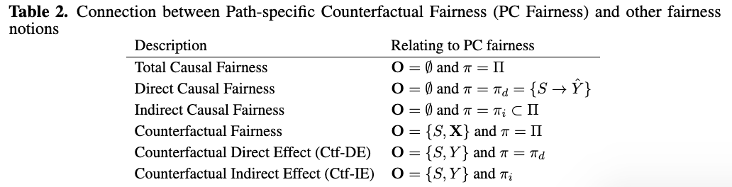
In [9], Wu et al. proposed path-specific counterfactual fairness (PC fairness) that covers the previously mentioned fairness notions. Letting $\Pi$ be all causal paths from $S$ to $Y$ in the causal graph and $\pi$ be a subset of $\Pi$, the path-specific counterfactual fairness metric is defined as follows.
Definition: Path-specific Counterfactual Fairness (PC Fairness)
Given a factual condition $\mathbf{O} = \mathbf{o}$ where $\mathbf{O} \subseteq {S, \mathbf{X}, Y }$ and a causal path set $\pi$, we achieve the PC fairness if:
$PCE{\pi}(s_1, s_0\mid \mathbf{o}) = P(y_{s_1 \vert \pi, s_0 \vert \overline{\pi}}\mid \mathbf{o}) - P(y_{s_0}\mid \mathbf{o}) =0$
where $s_1, s_0 \in { s^+, s^-}$.
In order to achieve path-specific counterfactual fairness in the running example, the application decision system needs to be able to discern the causal effect of the applicants gender being Female along the fair and unfair pathways, and to disregard the effect along the pathways that are unfair.
We point out that we can simply define the PC Fairness on a classifier by replacing outcome $Y$ with the predictor $\hat{Y}$ in the above equation. Previous causality-based fairness notions can be expressed as special cases of the PC fairness based on the value of $\mathbf{O}$ (e.g., $\emptyset$ or $S,{\mathbf{X}}$ ) and the value of $\pi$ (e.g., $\Pi$ or $\pi_d$). Their connections are summarised in Table 2 below, where $\pi_d$ contains the direct edge from $S$ to $\hat{Y}$, and $\pi_i$ is a path set that contains all causal paths passing through any redlining attributes. The notion of PC fairness also resolves new types of fairness, e.g., individual indirect fairness, which means discrimination along the indirect paths for a particular individual. Formally, individual indirect fairness can be directly defined and analyzed using PC fairness by letting $\mathbf{O}={S,\mathbf{X}}$ and $\pi=\pi_{i}$.
Proxy Fairness
In [10], Kilbertus et al. proposed proxy fairness. A proxy is a descendant of $S$ in the causal graph whose observable quantity is significantly correlated with $S$, but should not affect the prediction. An example of a proxy variable in our running admission case can be seen in the figure below.
Definition: Proxy Discrimination
A predictor $\hat{Y}$ exhibits no proxy discrimination based on a proxy $P$ if for all $p,p’$ we have:
$P(\hat{y}\mid do(P = p)) = P(\hat{Y}\mid do(P = p'))$
Intuitively, a predictor satisfies proxy fairness if the distribution of $\hat{Y}$ under two interventional regimes in which $P$ set to $p$ and $p’$ is the same. [10] presented the conditions and developed procedures to remove proxy discrimination given the structural equation model.
Justifiable Fairness
In [11], Salimi et al. presented a pre-processing approach for removing the effect of any discriminatory causal relationship between the marginalization attribute and classifier predictions by manipulating the training data to be non-discriminatory. The repaired training data can be seen as a sample from a hypothetical fair world.
Definition: $\mathbf{K}$-fair$
For a give set of variables $\mathbf{K}$, a decision function is said to be $\mathbf{K}$-fair with regards to $S$ if, for any context $\mathbf{K}=\mathbf{k}$ and any outcome $Y=y$, $P(y_{s_0, \mathbf{k}}) = P(y_{s_1,\mathbf{k}})$.
Note that the notion of $\mathbf{K}$-fair intervenes on both the marginalization attribute $S$ and variables $\mathbf{K}$. It is more fine-grained than proxy fairness, but it does not attempt to capture fairness at the individual level. The authors further introduced justifiable fairness for applications where the user can specify admissible (deconfounding) variables through which it is permissible for the marginalization attribute to influence the outcome. In our example, the admissible variable is the major.
Definition: Justifiable Fairness
A fairness application is justifiable fair if it is $\mathbf{K}$-fair with regarding to all supersets $\mathbf{K} \supseteq \mathbf{A}$ where $\mathbf{A}$ is the set of admissible variables.
Different from previous causality-based fairness notions, which require the presence of the underlying causal model, the justifiable fairness notion is based solely on the notion of intervention. The user only requires specification of a set of admissible variables and does not need to have a causal graph. The authors also introduced a sufficient condition for testing justifiable fairness that does not require access to the causal graph. However, with the presence of the causal graph, if all directed paths from $S$ to $Y$ go through an admissible attribute in $\mathbf{A}$, then the algorithm is justifiably fair. If the probability distribution is faithful to the causal graph, the converse also holds. This means that our running example is not justifiably fair since the paths from gender to admission has two paths: gender $\to$ major $\to$ admission and gender $\to$ admission.
Counterfactual Error Rate
Zhang and Bareinboim [2] developed a causal framework to link the disparities realized through equalized odds (EO) and the causal mechanisms by which the marginalization attribute $S$ affects change in the prediction $\hat{Y}$. EO, also referred to as error rate balance, considers both the ground truth outcome $Y$ and predicted outcome $\hat{Y}$. EO achieves fairness through the balance of the misclassification rates (false positive and negative) across different demographic groups. They introduced a family of counterfactual measures that allows one to explain the misclassification disparities in terms of the direct, indirect, and spurious paths from $S$ to $\hat{Y}$ on a structural causal model. Different from all previously discussed causality-based fairness notions, counterfactual error rate considers both $Y$ and $\hat{Y}$ in their counterfactual quantity.
Definition: Counterfactual Direct Error Rate
Given a SCM and a classifier $\hat{y}=f(\widehat{pa{}})$ where $\widehat{Pa{}}$ is a set of input features of the predictor, the counterfactual direct error rate ($ER^d$) for a sub-population $s,y$ (with prediction $\hat{y} \ne y)$ is defined as:
$ER^d_{s_0,s_1}(\hat{y}\mid s,y) = P(\hat{y}$$_{s_1,y,(\widehat{Pa{}}\backslash S)_{s_0,y}}\mid s,y) - P(\hat{y}$$_{s_0,y}\mid s,y)$
For an individual with the marginalization attribute $S=s$ and the true outcome $Y=y$, the counterfactual direct error rate calculates the difference of two terms. The first term is the prediction $\hat{Y}$ had $S$ been $s_1$, while keeping all the other features $\widehat{Pa{}}\backslash S$ at the level that they would attain had $S=s_0$ and $Y=y$, whereas the second term is the prediction $\hat{Y}$ the individual would receive had $S$ been $s_0$ and $Y$ been $y$.
Definition: Counterfactual Indirect Error Rate
Given a SCM and a classifier $\hat{y}=f(\widehat{pa{}})$, the counterfactual indirect error rate ($ER^i$) for a sub-population $s,y$ (with prediction $\hat{y} \ne y)$ is defined as:
$ER^i_{s_0,s_1}(\hat{y}\mid s,y) = P(\hat{y}$$_{s_0,y,(\hat{PA}\backslash S)_{s_1,y}}\mid s,y) - P(\hat{y}$$_{s_0,y}\mid s,y)$
Definition: Counterfactual Spurious Error Rate
Given a SCM and a classifier $\hat{y}=f(\widehat{pa{}})$, the counterfactual spurious error rate ($ER^s$) for a sub-population $s,y$ (with prediction $\hat{y} \ne y)$ is defined as:
$ER^s_{s_0,s_1}(\hat{y}\mid y) = P(\hat{y}$$_{s_0,y}\mid s_1,y) - P(\hat{y}$$_{s_0,y}\mid s_0,y)$
The counterfactual spurious error rate can be read as “for two demographics $s_0$, $s_1$ with the same true outcome $Y=y$, how would the prediction $\hat{Y}$ differ had they both been $s_0$, $y$?” For a graphical depiction of these measures, we refer interested reader to the tutorial by Bareinboim, Zhang, and Plecko [12].
Building on these measures, Zhang and Bareinboim [2] derived the causal explanation formula for the error rate balance. The equalized odds notion constrains the classification algorithm such that its disparate error rate is equal to zero across different demographics.
Definition: Error Rate Balance
The error rate (ER) balance is given by:
$ER_{s_0, s_1}(\hat{y}\mid y) = P(\hat{y}\mid s_1,y) - P(\hat{y}\mid s_0,y)$
Theorem: Causal Explanation Formula of Equalized Odds
For any $s_0$, $s_1$, $\hat{y}$, $y$, we have the following relationship:
$ER_{s_0,s_1}(\hat{y}\mid y) = ER^d_{s_0,s_1}(\hat{y}\mid s_0,y) - ER^i_{s_1,s_0}(\hat{y}\mid s_0,y) - ER^s_{s_1,s_0}(\hat{y}\mid y)$
The above theorem shows that the total disparate error rate can be decomposed into terms, each of which estimates the adverse impact of its corresponding discriminatory mechanism.
Individual Equalized Counterfactual Odds
In [13], Pfohl et al. proposed the notion of individual equalized counterfactual odds that is an extension of counterfactual fairness and equalized odds. The notion is motivated by clinical risk prediction and aims to achieve equal benefit across different demographic groups.
Definition: Individual Equalized Counterfactual Odds
Given a factual condition $\mathbf{O} = \mathbf{o}$ where $\mathbf{O} \subseteq {\mathbf{X}, Y }$, predictor $\hat{Y}$ achieves the individual equalized counterfactual odds if:
$P(\hat{y}$$_{s_1} \mid \mathbf{o},y_{s_1}, s_0) - P(\hat{y}$$_{s_0} \mid \mathbf{o}, y_{s_0}, s_0) =0$
where $s_1, s_0 \in { s^+, s^-}$.
The notion implies that the predictor must be counterfactually fair given the outcome $Y$ matching the counterfactual outcome $y_{s_0}$. This is different than the normal counterfactual fairness calculation, which requires the prediction to be equal across the factual/counterfactual pairs, without caring if those pairs have the same outcome prediction. Therefore, in addition to requiring predictions to be equal across factual/counterfactual samples, those samples must also share the same value of the actual outcome $Y$. In other words, it considers the desiderata from both counterfactual fairness and equalized odds. For our running example, this is an extension of the discussion under the definition for counterfactual fairness, in which we now require that $\hat{y}\(_{s_0} = \hat{y}\)_{s_1}$.
Fair on Average Causal Effect
In [14], Khademi et al. introduced two definitions of group fairness: fair on average causal effect (FACE), and fair on average causal effect on the treated (FACT) based on the Rubin-Neyman potential outcomes framework. Let $Y_i(s)$ be the potential outcome of an individual data point $i$ had $S$ been $s$.
Definition: Fair on Average Causal Effect (FACE)
A decision function is said to be fair, on average over all individuals in the population, with respect to $S$, if $\mathbb{E}[Y_i(s_1) - Y_i(s_0)] =0$.
FACE considers the average causal effect of the marginalization attribute $S$ on the outcome $Y$ at the population level and is equivalent to the expected value of the $TCE(s_1, s_0)$ in the structural causal model.
Definition: Fair on Average Causal Effect on the Treated (FACT)
A decision function is said to be fair with respect to $S$, on average over individuals with the same value of $s_1$, if $\mathbb{E}[Y_i(s_1) - Y_i(s_0)\mid S_i =s_1] =0$.
FACT focuses on the same effect at the group level. This is equivalent to the expected value of $ETT_{s_1,s_0}(Y)$. The authors used inverse probability weighting to estimate FACE and use matching methods to estimate FACT.
Equality of Effort
In [15], Huang et al. developed a fairness notation called equality of effort. When applied to the example, we have a dataset with $N$ individuals with attributes $(S, T, \mathbf{X}, Y)$ where $S$ denotes the marginalization attribute gender with domain values ${ s^+, s^-}$, $Y$ denotes a decision attribute admission with domain values ${ y^+, y^-}$, $T$ denotes a legitimate attribute such as test score, and $\mathbf{X}$ denotes a set of covariates. For an individual $i$ in the dataset with profile $(s_{i}, t_{i}, x_{i}, y_{i})$, they may ask the counterfactual question, how much they should improve their test score such that the probability of their admission is above a threshold $\gamma$ (e.g., $80\%$).
Definition: $\gamma$-Minimum Effort
For individual $i$ with value $(s_{i}, t_{i}, x_{i}, y_{i})$, the minimum value of the treatment variable to achieve $\gamma$-level outcome is defined as:
$\Psi_i (\gamma) = \arg\!\min_{t\in T} \big\{ \mathbb{E}[Y_i(t)] \geq \gamma) \}$
and the minimum effort to achieve $\gamma$-level outcome is $\Psi_i (\gamma)- t_{i}$.
If the minimal change for individual $i$ has no difference from that of counterparts (individuals with similar profiles except the marginalization attribute), individual $i$ achieves fairness in terms of equality of effort. As $Y_i(t)$ cannot be directly observed, we can find a subset of users, denoted as $I$, each of whom has the same (or similar) characteristics ($\mathbf{x}$ and $t$) as individual $i$. $I^$ denotes the subgroup of users in $I$ with the marginalization attribute value $s^$ where $* \in {+,-}$ and $\mathbb{E}[Y_{I^}(t)]$ denotes the expected outcome under treatment $t$ for the subgroup $I^$.
Definition: $\gamma$-Equal Effort Fairness
For a certain outcome level $\gamma$, the equality of effort for individual $i$ is defined as:
$\Psi_{I^+}(\gamma) = \Psi_{I^-}(\gamma)$
where $\Psi_{I^+}(\gamma) = \arg\min_{t\in T} {\mathbb{E}[Y_{I^+}(t)] \geq \gamma }$ is the minimal effort needed to achieve $\gamma$ level of outcome variable within the subgroup $+$ (or equivalently $-$.
Equal effort fairness can be straightforwardly extended to the system (group) level by replacing $I$ with the whole dataset $D$ (or a particular group). Different from previous fairness notations that mainly focus on the the effect of the marginalization attribute $S$ on the decision attribute $Y$, the equality of effort instead focuses on to what extend the treatment variable $T$ should change to make the individual achieve a certain outcome level. This notation addresses the concerns whether the efforts that would need to make to achieve the same outcome level for individuals from the marginalized group and the efforts from the non-marginalized group are different. For instance, if we have two students with the same credentials minus their gender, and the Female student was required to raise their test score significantly more than the Male, then we do not achieve equal effort fairness.
Technical Pitfalls of Causality-based Fairness
Causality provides a conceptual and technical framework for measuring and mitigating unfairness by using the causal effect on a decision from hypothetical interventions on marginalization attributes such as gender. Despite the benefits of causality-based notions over statistical-based ones, there have been technical challenges in applying causality for fair machine learning in practice. One common challenge is the validity of the assumptions in causal modeling. The majority of research on causal fairness is based on SCM which represents the causal relationships between variables via structural equations and a directed acyclic graph (DAG). In practice, learning structural equations and constructing the DAG model from observational data is a challenging task and often relies on strong assumptions such as the Markov property, faithfulness, and sufficiency [16]. Simply speaking, the Markov property requires that all nodes are independent of their non-descendants when conditioned on their parents; faithfulness requires all conditional independent relationships in the true underlying distribution are represented in the DAG; and sufficiency requires any pair of nodes in the DAG has one common external cause (confounder). These assumptions help narrow down the model space, however, they may not hold in the causal process or the sampling process that generates the observed data.
Another common challenge of causality-based fairness notions based on SCMs is identifiability, i.e., whether they can be uniquely measured from observational data. As causality-based fairness notions are defined based on different types of causal effects, such as total effect on interventions, direct/indirect discrimination on path-specific effects, and counterfactual fairness on counterfactual effects, their identifiability depends on the identifiability of these causal effects. Unfortunately, in many situations these causal effects are unidentifiable. Hence identifiability is a critical barrier for causality-based fairness to be applied to real applications. In the causal inference field, researchers have studied the reasons for unidentifiability and identified the corresponding structural patterns such as the existence of the “kite graph”, the “w graph”, or the “hedge graph”. We refer readers who are interested in learning the specifics of identifiability theory and criteria, and how they can be used to decide the applicability of causality-based fairness metrics to [17]. We also refer readers to [9] for a summary of unidentifiable situations and approximation techniques to derive bounds of causal effects.
The potential outcome framework does not require the causal graph. However, as discussed in the previous post, it relies on three assumptions. SUTVA is a non-interference assumption which may not hold in many real world applications. For example, a loan officer’s decision to proceed with one application may be influenced by previous applications. In this case, SUTVA is violated. When the strong ignorability assumption does not hold, there exist hidden confounders. Although we can leverage mediating features or proxies to estimate treatment effects [18], the lack of accuracy guarantee hinders the applicability of causal fairness.