Causality

2022, Mar 12    

The goal of standard statistical analysis is to find associations among variables in order to estimate and update probabilities of past and future events in light of new information. Causal inference analysis, on the other hand, aims to infer probabilities under conditions that are changing due to outside interventions [1]. Causal inference analysis (or simply causal inference) presents a formal language that allows us to draw conclusions that a specific intervention caused the observed outcome. For example, that the rain caused the grass to be wet or that taking Claritin caused your seasonal allergies to go away.

There are many different theories for understanding causality, such as regularity theories, mechanistic theories, probabilistic approaches, counterfactual reasoning, and the manipulationist approaches that house the interventionalist theories of which Pearl’s structural causal model and Rubin’s potential outcome frameworks belong to. In this post, I will mainly focus on the interventionalist approaches of both Pearl and Rubin as they are the most widely used frameworks for causal inference.

A Primer on Causal Inference

I will begin by giving a short introduction of the terminology and concepts of the causal machine learning field. Throughout this section we will use the running example of determining whether a patient will survive a specific sickness ( $D$ ) based on the initial severity of the disease ($S$) and the treatment administered ( $T$ ). Three different causal diagrams showing this scenario can be seen below.

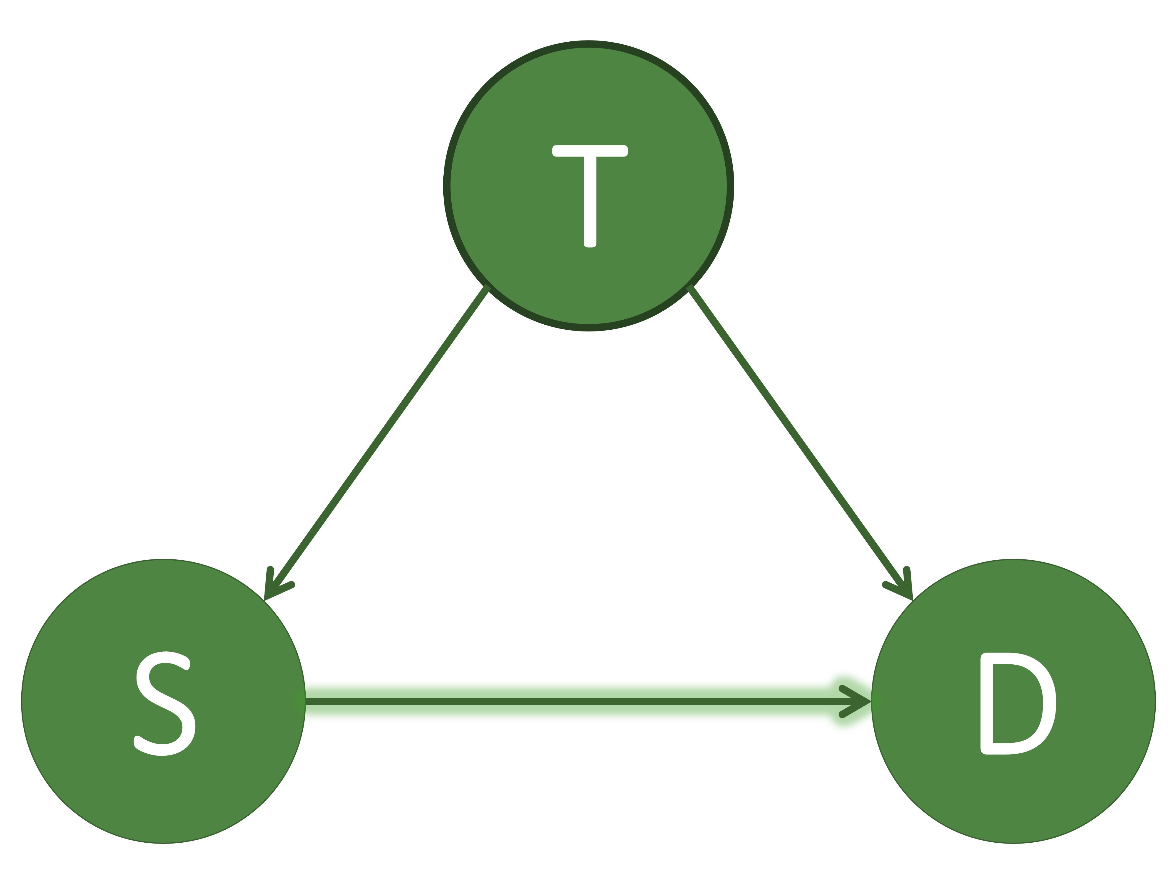
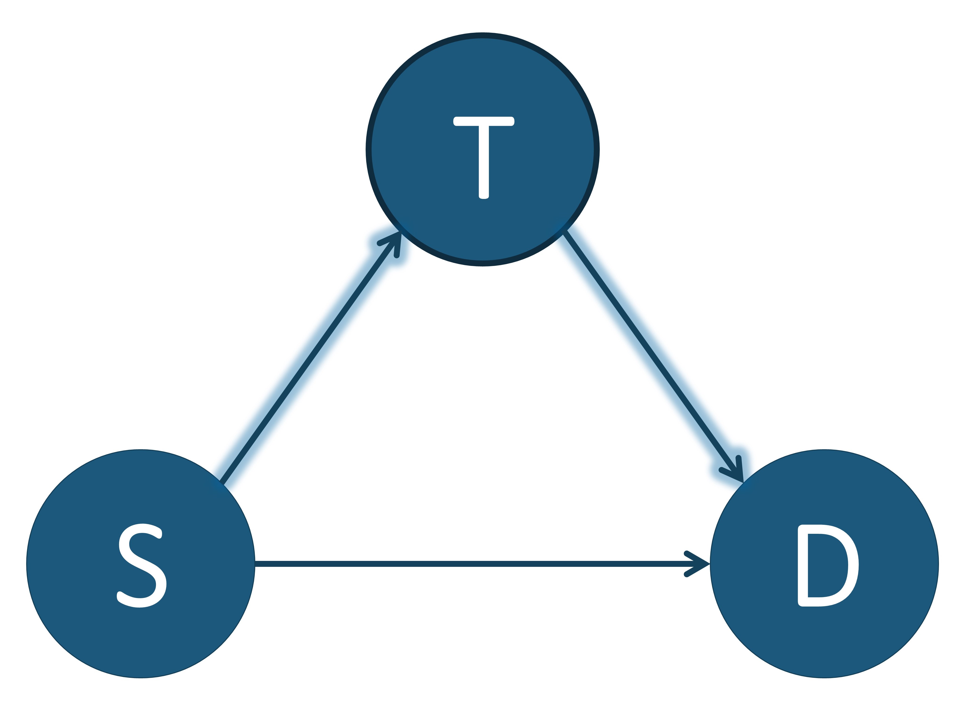
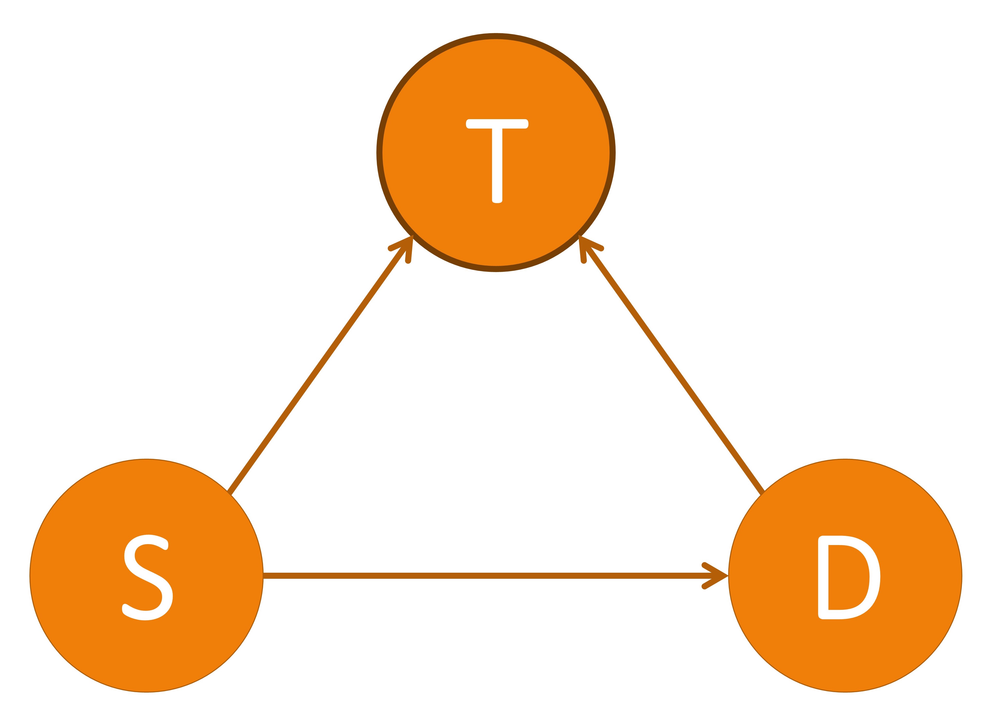
These three causal models showing $T$ as a confounder, mediator, and collider. $T$: treatment, $S$: severeness, $D$: survival. In (a), $T$ is a confounder since it impacts both the input variable $S$ and the output variable $D$. In (b), $T$ is a mediator since it lies between the input variable $S$ and the output variable $D$ in one possible path. In (c), $T$ is a collider since it is influenced by both $S$ and $D$. An example of a direct path is shown in (a) by the arrow highlighted in green going from $S$ to $D$. An example of an indirect path is shown in (b) by the arrows highlighted in blue traveling from $S$ to $D$ through $T$.

There are multiple different variable types in causal inference, where each variable represents the occurrence (or non-occurrence) of an event, a property of an individual or of a population of individuals, or a quantitative value. The output variable is the particular variable that we want to affect by administering interventions, or treatments, on specific treatment variables. When administering the treatment on the treatment variable, we hold all other variable values unchanged. A variable is considered a confounder if it affects both the input and the outcome variables since it causes a spurious association between the two variables. When performing causal analysis, confounding variables must be controlled for since they can incorrectly imply that one variable caused another. An example of a confounder can be seen in the first figure above. When a path such as $S \to T \to D$ exists, we call $T$ the mediator variable since it contributes to the overall effect of $S$ on $D$. An example of this can be seen in the middle image. Finally, a collider is a variable that is causally influenced by two or more variables, and it is named as such since it appears that the arrow heads from the incoming variables “collide” at the node. This can be seen in the last image. It is important to mention that “colliders aren’t confounders” and that we should not condition on a collider since it can create a correlation between two previously uncorrelated variables [2].

In addition to there being different types of variables, there are two main ways that one variable can cause an effect on another. The first way is a direct effect, where one variable directly affects the output variable. In order to measure the direct effect of a variable on the output variable all other possible paths (besides the direct path) need to be “disabled” or controlled. For example, in the first photo above, we can measure the direct effect $S$ has on $D$ by making the treatment $T$ be the same for all individuals. The other type of effect is called an indirect effect. This occurs when the effect of a variable on the output variable is transmitted through a mediator along an indirect path. An example of this can be seen in the second image above by the arrows highlighted in blue. In this setting, the path from $S$ to $D$ is mediated by the variable $T$.

Using the foundation of causal inference formed above, we can now introduce the two frameworks that are fundamental to causality-based machine learning fairness notions. The first framework is the structural causal model (SCM) framework proposed by Pearl [3], and the second is the potential outcome (PO) framework proposed by Rubin [4]. While we will discuss the two frameworks separately since they have different assumptions of the amount of information available, they are logically equivalent. However, we can derive a PO from a SCM, but we cannot derive a SCM from a PO alone because SCMs make more assumptions about the relationships between the variables that cannot be derived from a PO [2].

Throughout the post I use the following notation conventions. An uppercase letter denotes a variable, e.g., $X$; a bold uppercase letter denotes a set of variables, e.g., $\mathbf{X}$; a lowercase letter denotes a value or a set of values of the corresponding variables, e.g., $x$ and $\mathbf{x}$; $PA_{X}$ denotes the set of variables that directly determine the value of a variable $X$ (often times called the parents of $X$); and $pa_{X}$ denotes the values of X’s parents. We also note that we will use the terms ‘factors’ and ‘variables’ interchangeably throughout the rest of the post.

Structural Causal Model - (SCM)

The structural causal model (SCM) was first proposed by Judea Pearl in [3]. Pearl believed that by understanding the logic behind causal thinking, we would be able to emulate it on a computer to form more realistic artificial intelligence [5]. He proposed that causal models would give the ability to “anchor the elusive notions of science, knowledge, and data in a concrete and meaningful setting, and will enable us to see how the three work together to produce answers to difficult scientific questions,’’ [5]. We recount the important details of SCMs below.

Definition: Structural Causal Model [3]

A structural causal model $\mathcal{M}$ is represented by a quadruple $\langle \mathbf{U}, \mathbf{V}, \mathbf{F}, P(\mathbf{U}) \rangle$ where:

• $\mathbf{U}$ is a set of exogenous (external) variables that are determined by factors outside the model.
• $\mathbf{V}$ is a set of endogenous (internal) variables that are determined by variables in $\mathbf{U}\cup\mathbf{V}$ , i.e., $\mathbf{V}$ ‘s values are determined by factors within the model.
• $\mathbf{F}$ is a set of structural equations from $\mathbf{U} \cup \mathbf{V} \to \mathbf{V}$, i.e., $v_i=f_{v_i} (pa_{v_i}, u_i )$ for each $v_i \in \mathbf{V}$ where $u_V$ is a random disturbance distributed according to $P(U)$. In other words, $f_{v_i}(\cdot)$ is a structural equation that expresses the value of each endogenous variable as a function of the values of the other variables in $\mathbf{U}$ and $\mathbf{V}$.
• $P(\mathbf{U})$ is a joint probability distribution defined over $\mathbf{U}$.

In general, $f_{v_i}(\cdot)$ can be any type of equation. But, we will discuss $f_{v_i}(\cdot)$ as a non-linear, non-parametric generalization of the standard linear equation $v_i = \sum_{k\in PA_{i}}\alpha_{ik}v_k+u_i, \;i=1,\dots,n$ , where $\alpha$ is a coefficient. If all exogenous variables in $\mathbf{U}$ are assumed to be mutually independent, meaning that each variable in $\mathbf{U}$ is independent of any combination of other variables in $\mathbf{U}$, then the causal model is called a Markovian model; otherwise, it is called a semi-Markovian model.

The causal model $\mathcal{M}$ is associated with a causal graph $\mathcal{G} = \langle \mathcal{V}, \mathcal{E} \rangle$ where $\mathcal{V}$ is a set of nodes (otherwise known as vertices) and $\mathcal{E}$ is a set of edges. Each node of $\mathcal{V}$ corresponds to an endogenous variable of $\mathbf{V}$ in $\mathcal{M}$. Each edge in $\mathcal{E}$, denoted by a directed arrow $\rightarrow$, points from a node $X\in \mathbf{U} \cup \mathbf{V}$ to a different node $Y\in \mathbf{V}$ if $f_Y$ uses values of $X$ as input. A causal path from $X$ to $Y$ is a directed path from $X$ to $Y$. For example, in the first image below, $\text{Age} (A)\to\text{Severeness}(S)\to\text{Survival}(D)$ is a causal path from Age to Survival. To make the causal graph easier to analyze, the exogenous variables are normally removed from the graph. In a Markovian model, exogenous variables can be directly removed without losing any vital information. In a semi-Markovian model, after removing exogenous variables, we also need to add dashed bi-directional edges between the children of correlated exogenous variables to indicate the existence of an unobserved common cause, i.e., a hidden confounder. For instance, if in the first image below we treated gender as an exogenous variable, we could remove it from the graph by adding a bi-directional dashed line, as shown in the second image.

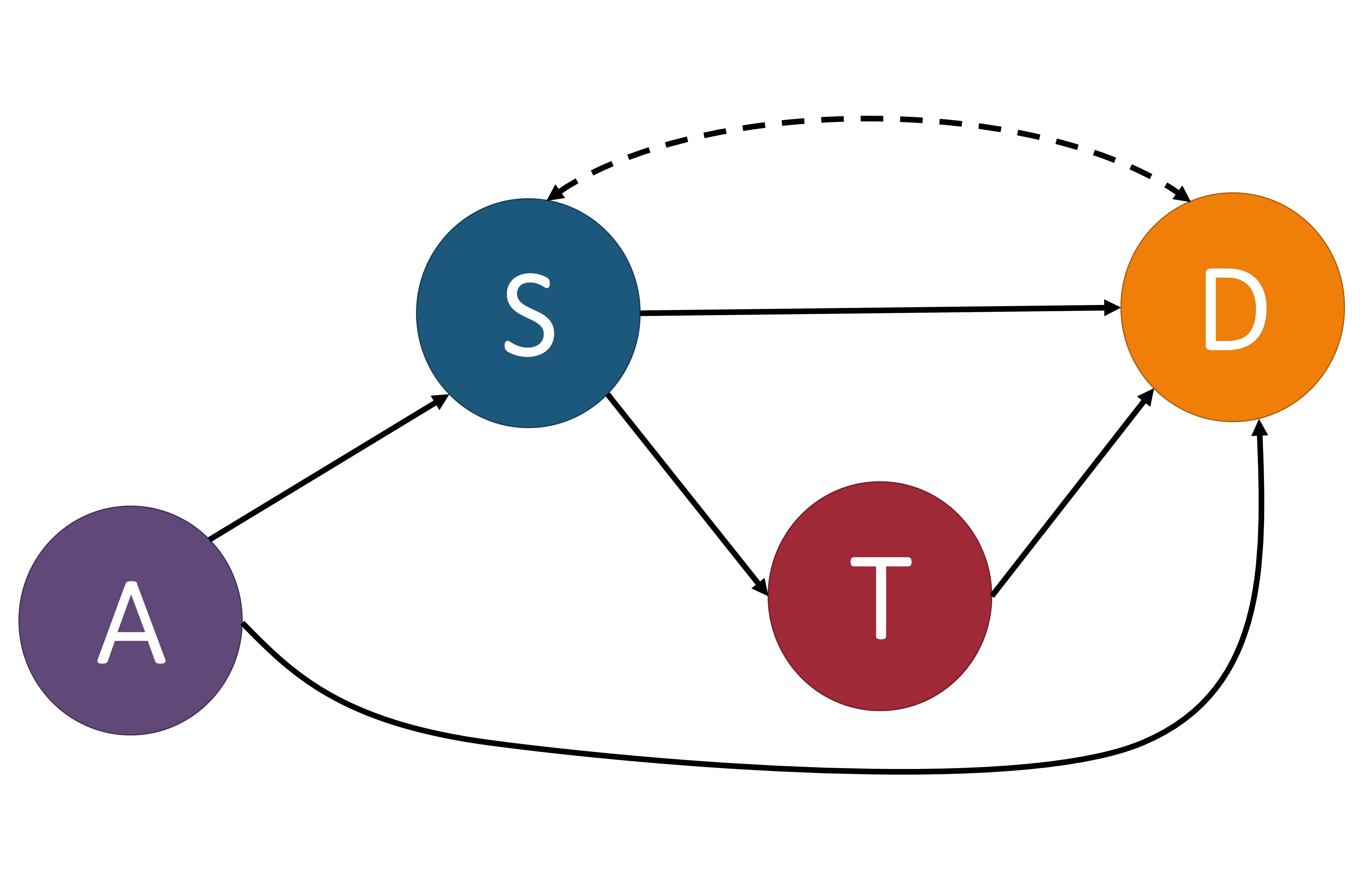
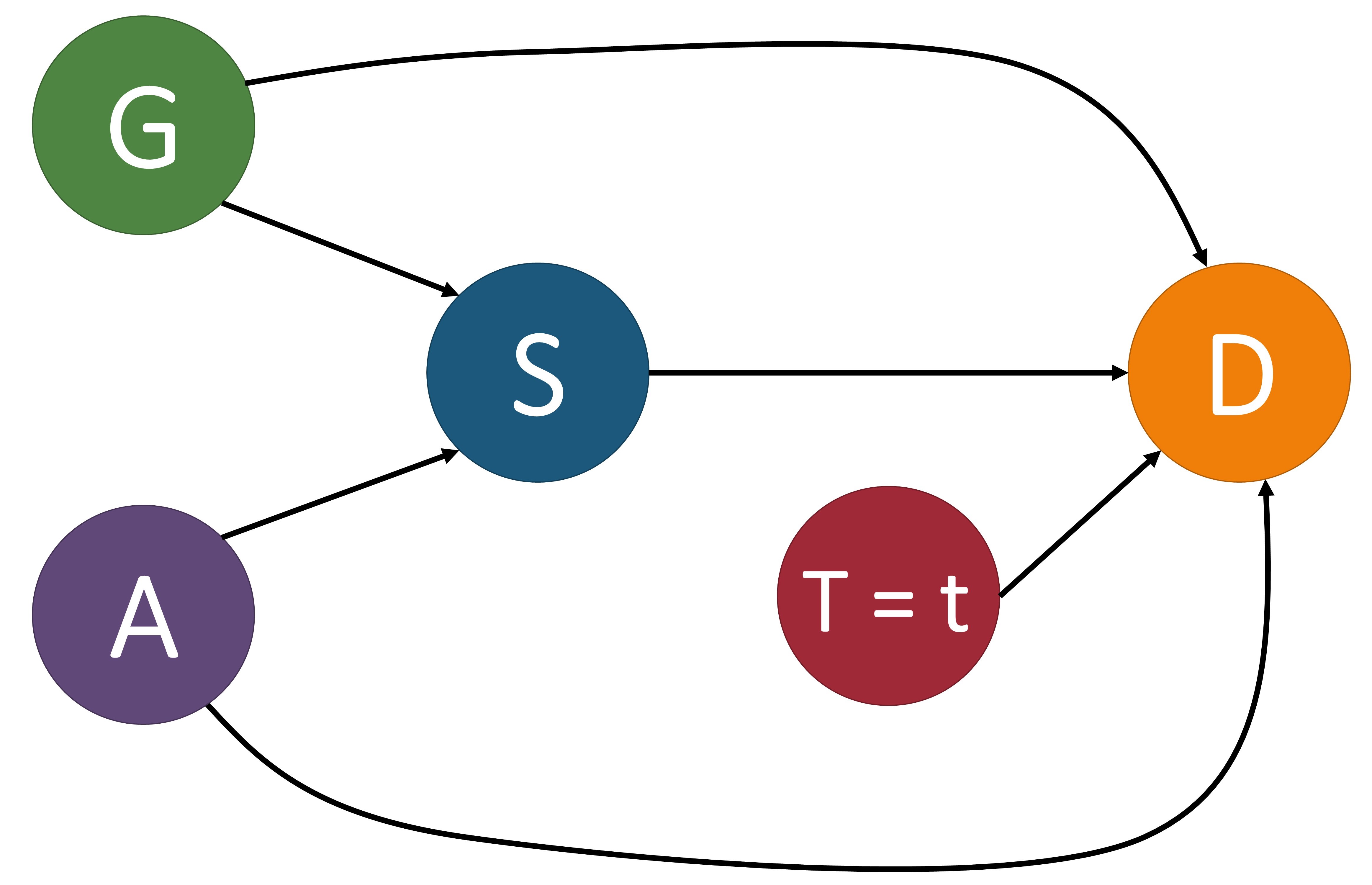
These images of a structural causal models depict the relationships between variables that determine the survival of some disease. $G$: gender, $A$: age, $S$: severeness, $T$: treatment, $D$: survival. In (a), we include the exogenous variable gender and in (b) we show it removed by adding a bi-directional dashed line between $S$ and $D$ since this is a semi-Markovian model. In (c), we perform an intervention on variable $T$ by setting it equal to $t$.

Quantitatively measuring causal effects in a causal model is made possible by using the $do$-operator [3] which forces some variable $X$ to take on a certain value $x$. The $do$-operator can be formally denoted by $do(X = x)$ or $do(x)$. By substituting a value for another using the $do$-operator, we break the natural course of action that our model captures [2]. In a causal model $\mathcal{M}$, the intervention $do(x)$ is defined as the substituting of the structural equation $X=f_{X}(PA_{X}, U_X)$_ with $X=x$. This change corresponds to a modified causal graph that has removed all edges coming into $X$ and in turn sets $X$ to $x$. An example of this can be seen in the third image above. For an observed variable $Y$ which is affected by the intervention, its interventional variant is denoted by $Y_{x}$. The distribution of $Y_{x}$, also referred to as the post-intervention distribution of $Y$ under $do(x)$, is denoted by $P(Y_x=y)$ or simply $P(y_x)$.

Similarly, the intervention that sets the value of a set of variables $\mathbf{X}$ to $\mathbf{x}$ is denoted by $do(\mathbf{X} = \mathbf{x})$. The post-intervention distribution of all other attributes $\mathbf{Y}=\mathbf{V}\backslash \mathbf{X}$, i.e., $P(\mathbf{Y}=\mathbf{y}\mid do(\mathbf{X}=\mathbf{x}))$, or simply $P(\mathbf{y}\mid do(\mathbf{x}))$, can be computed by the truncated factorization formula [3]:

$P(\mathbf{y}\mid do(\mathbf{x})) = \prod_{Y\in \mathbf{Y}}P(y\mid PA_{}(Y))\delta_{\mathbf{X}=\mathbf{x}}$

where $\delta_{\mathbf{X}=\mathbf{x}}$ assigns attributes in $\mathbf{X}$ involved in the term with the corresponding values in $\mathbf{x}$. Specifically, the post-intervention distribution of a single attribute $Y$ given an intervention on a single attribute $X$ is given by:

$P(y\mid do(x)) = \sum_{\mathbf{V}\backslash \{X,Y\},Y=y}\prod_{V\in \mathbf{V}\backslash \{X\}}P(v\mid PA_{}(V))\delta_{X=x}$

where the summation is a marginalization that traverses all value combinations of $\mathbf{V}\backslash {X,Y}$. Note that $P(y\mid do(x))$ and $P(y\mid x)$ are not equal. In other words, the probability distribution representing the statistical association ( $P(y\mid x)$ ) is not equivalent to the interventional distribution ( $P(y\mid do(x))$ ).

Above I mentioned that there were only two types of effects: direct and indirect. This is a slight relaxation of what can be measured in a SCM. By using the $do$-operator, we can measure multiple types of effects that one variable has on another, including: total causal effect, controlled direct effect, natural direct/indirect effect, path-specific effect, effect of treatment on the treated, counterfactual effect, and path-specific counterfactual effect. I detail their definitions below.

Definition: Total Causal Effect [3]

The total causal effect (TCE) of the value change of $X$ from $x_0$ to $x_1$ on $Y=y$ is given by:

$TCE(x_1, x_0) = P(y_{x_1}) - P(y_{x_0})$

The total causal effect is defined as the effect of $X$ on $Y$ where the intervention is transferred along all causal paths from $X$ to $Y$. In contrast with the TCE, the controlled direct effect (CDE) measures the effect of $X$ on $Y$ while holding all the other variables fixed.

Definition: Controlled Direct Effect

The controlled direct effect (CDE) of the value change of $X$ from $x_0$ to $x_1$ on $Y=y$ is given by:

$\mathrm{CDE}(x_1, x_0) = P(y_{x_1,\mathbf{z}}) - P(y_{x_0,\mathbf{z}})$

where $\mathbf{Z}$ is the set of all other variables.

In [6], Pearl introduced the causal mediation formula which allowed the decomposition of total causal effect into natural direct effect (NDE) and natural indirect effect (NIE).

Definition: Natural Direct Effect

The natural direct effect (NDE) of the value change of $X$ from $x_0$ to $x_1$ on $Y=y$ is given by:

$\mathrm{NDE}(x_1, x_0) = P(y_{x_1, \mathbf{Z}_{x_0}}) - P(y_{x_0})$

where $\mathbf{Z}$ is the set of mediator variables and the first term in the subtraction is the probability of $Y=y$ had $X$ been $x_1$ and had $\mathbf{Z}$ been the value it would naturally take if $X=x_0$. In the causal graph, $X$ is set to $x_1$ in the direct path $X \rightarrow Y$ and is set to $x_0$ in all other indirect paths.

Definition: Natural Indirect Effect

The natural indirect effect (NIE) of the value change of $X$ from $x_0$ to $x_1$ on $Y=y$ is given by:

$\mathrm{NIE}(x_1, x_0) = P(y_{x_0, \mathbf{Z}_{x_1}}) - P(y_{x_0})$

NDE measures the direct effect of $X$ on $Y$ while NIE measures the indirect effect of $X$ on $Y$. NDE differs from CDE since the mediators $\mathbf{Z}$ are set to $\mathbf{Z}_{x_0}$ in NDE and not in CDE. In other words, the mediators are set to the value that they would have naturally attained under the reference condition $X=x_0$.

One main problem with NIE is that it does not enable the separation of “fair” (explainable discrimination) and “unfair” (indirect discrimination) effects (we will expound on the definitions of discrimination in the following sections). Path-specific effect [3], which is an extension of TCE in the sense that the effect of the intervention is transmitted only along a subset of the causal paths from $X$ to $Y$, fixes this issue. Let $\pi$ denote a subset of the possible causal paths. The $\pi$-specific effect considers a counterfactual situation where the effect of $X$ on $Y$ with the intervention is transmitted along $\pi$, while the effect of $X$ on $Y$ without the intervention is transmitted along paths not in $\pi$.

Definition: Path-specific Effect [7]

Given a causal path set $\pi$, the $\pi$ -specific effect ( $PE_{\pi}$ ) of the value change of $X$ from $x_0$ to $x_1$ on $Y=y$ through $\pi$ (with reference $x_0$) is given by:

$PE_{\pi}(x_1, x_0) = P(y_{x_1 \vert \pi, x_0 \vert \overline{\pi}}) - P(y_{x_0})$

where $ P(Y_{ x_1 \vert \pi, x_0 \vert \overline{\pi} }) $ represents the post-intervention distribution of $Y$ where the effect of intervention $do(x_1)$ is transmitted only along $\pi$ while the effect of reference intervention $do(x_0)$ is transmitted along the other paths.

In addition to $PE_{\pi}$ being an extension of TCE, they are further connected in that : 1) if $\pi$ contains all causal paths from $X$ to $Y$ , then $PE_{\pi}(x_{1},x_{0})=\mathrm{TCE}(x_{1},x_{0})$ , and 2) for any $\pi$ , we have $PE_{\pi}(x_{1},x_{0}) + (-PE_{\overline{\pi}}(x_{0},x_{1})) = \mathrm{TCE}(x_{1},x_{0})$ where $\overline{\pi}$ represents the paths not in $\pi$ .

The above definitions for TCE and $PE_{\pi}$ consider the average causal effect over the entire population without using any prior observations. In contrast, the effect of treatment on the treated considers the effect on a sub-population of the treated group.

Definition: Effect of Treatment on the Treated

The effect of treatment on the treated (ETT) of intervention $X=x_1$ on $Y=y$ (with baseline $x_0$) is given by:

$\mathrm{ETT}_{x_1, x_0} = P(y_{x_1\mid x_0}) - P(y\mid x_0)$

where $P(y_{x_1\mid x_0})$ represents the counterfactual quantity that read as “the probability of $Y$ would be $y$ had $X$ been $x_1$, given that in the actual world, $X=x_0$.’’

If we have certain observations about a subset of attributes $\mathbf{O}=\mathbf{o}$ and use them as conditions when inferring the causal effect, then the causal inference problem becomes a counterfactual inference problem. This means that the causal inference is performed on the sub-population specified by $\mathbf{O}=\mathbf{o}$ only. Symbolically, conditioning the distribution of $Y_{x}$ on factual observation $\mathbf{O}=\mathbf{o}$ is denoted by $P(y_{x}\mid \mathbf{o})$. The counterfactual effect is defined as follows.

Definition: Counterfactual Effect [8]

Given a factual condition $\mathbf{O}=\mathbf{o}$, the counterfactual effect (CE) of the value change of $X$ from $x_0$ to $x_1$ on $Y=y$ is given by:

$\mathrm{CE}(x_1, x_0\mid \mathbf{o}) = P(y_{x_1} \mid \mathbf{o}) - P(y_{x_0} \mid \mathbf{o})$

In [9], the authors present a general representation of causal effects, called path-specific counterfactual effect, which considers an intervention on $X$ transmitted along a subset of causal paths $\pi$ to $Y$, conditioning on observation $\mathbf{O}=\mathbf{o}$.

Definition: Path-specific Counterfactual Effect

Given a factual condition $\mathbf{O}=\mathbf{o}$ and a causal path set $\pi$, the path-specific counterfactual effect (PCE) of the value change of $X$ from $x_0$ to $x_1$ on $Y=y$ through $\pi$ (with reference $x_0$) is given by:

$\mathrm{PCE}_{\pi}(x_1, x_0\mid \mathbf{o}) = P(y_{x_1 \vert \pi, x_0 \vert \overline{\pi}}\mid \mathbf{o}) - P(y_{x_0}\mid \mathbf{o})$

Potential Outcome Framework

The potential outcome framework [4], also known as Neyman-Rubin potential outcomes or the Rubin causal model, has been widely used in many research areas to perform causal inference since it is often easier to apply than SCM. This is because SCMs, in general, encode more assumptions about the relationships between variables and formulating a valid SCM can require domain knowledge that is not available[2]. The PO model, in contrast, is generally easier to apply since there is a broad set of statistical estimators of causal effects that can be readily applied to pure observational data.

PO refers to the outcomes one would see under each possible treatment option for a variable. Let $Y$ be the outcome variable, $T$ be the binary or multiple valued treatment variable, and $\mathbf{X}$ be the pre-treatment variables (covariates). Note that pre-treatment variables are the ones that are not affected by the treatment. On the other hand, the post-treatment variables, such as the intermediate outcome, are affected by the treatment.

Definition: Potential Outcome

Given the treatment $T = t$ and outcome $Y=y$, the potential outcome of the individual $i$, $Y_i(t)$, represents the outcome that would have been observed if the individual $i$ had received treatment $t$.

The potential outcome framework relies on three main assumptions:

1. Stable Unit Treatment Value Assumption (SUTVA): requires the potential outcome observation on one unit be unaffected by the particular assignment of treatments to other units.
2. Consistency Assumption: requires that the value of the potential outcomes would not change no matter how the treatment is observed or assigned through an intervention.
3. Strong Ignorability (unconfoundedness) Assumption: is equal to the assumption that there are no unobserved confounders.

Under these assumptions, causal inference methods can be applied to estimate the potential outcome and treatment effect given the information of the treatment variable and the pre-treatment variables. We refer interested readers to the survey [10] for various causal inference methods, including re-weighting, stratification, matching based, and representation based methods.

In practice, only one potential outcome can be observed for each individual, while in theory, all of the different possible outcomes still exist. The observed outcome is called the factual outcome and the remaining unobserved potential outcomes are the counterfactual outcomes. The potential outcome framework aims to estimate potential outcomes under different treatment options and then calculate the treatment effect. The treatment effect can be measured at the population, treated group, subgroup, and individual levels.

As we did above for SCM, we will now recount popular ways to measure the treatment effect in PO. In addition, without loss of generality, in the following discussion we assume that the treatment variable is binary.

Definition: Average Treatment Effect

Given the treatment $T = t$ and outcome $Y=y$, the average treatment effect (ATE) is defined as:

$\mathrm{ATE} = \mathbb{E}[Y(t')-Y(t)]$

where $Y(t’)$ and $Y(t)$ are the potential outcome and the observed control outcome of the whole population, respectively. \end{definition}

Definition: Average Treatment Effect on the Treated

Given the treatment $T = t$ and outcome $Y=y$, the average treatment effect on the treated group ($ATT$) is defined as:

$\mathrm{ATT} = \mathbb{E}[Y(t')-Y(t)\mid T=t]$

The ATE answers the question of how, on average, the outcome of interest $Y$ would change if everyone in the population of interest had been assigned to a particular treatment $t’$ relative to if they had received another treatment $t$. The ATT, on the other hand, details how the average outcome would change if everyone who received one particular treatment $t$ had instead received another treatment $t’$.

Definition: Conditional Average Treatment Effect

Given the treatment $T = t$ and outcome $Y=y$, the conditional average treatment effect ($CATE$) is defined as:

$\mathrm{CATE} = \mathbb{E}[Y(t')-Y(t)\mid \mathbf{W}={w}]$

where $\mathbf{W}$ is a subset of variables defining the subgroup.

Definition: Individual Treatment Effect

Given the treatment $T = t$ and outcome $Y=y$, the individual treatment effect (ITE) is defined as:

$\mathrm{ITE} = \mathbb{E}[Y_i(t')-Y_i(t)]$

where $Y_i(t’)$ and $Y_i(t)$ are the potential outcome and the observed control outcome of individual $i$, respectively.