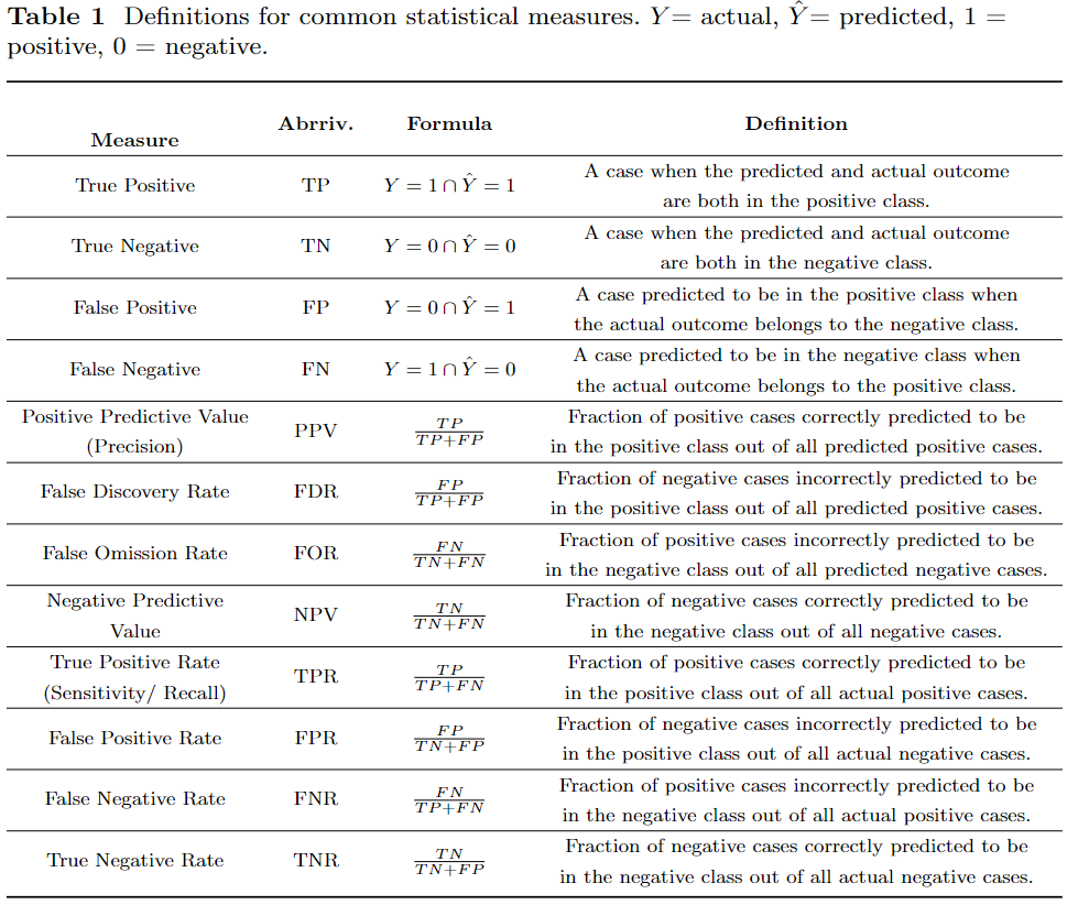
Many of the proposed fair machine learning metrics have groundings in statistics [1]. For example, statistical parity depends on the measurement of raw positive classification rates; equalized odds depends on false positive and false negative rates; and predictive parity depends on true positive rates. The use of statistical measures is attractive because they are relatively simple to measure and definitions built using statistical measures can usually be achieved without having to make any assumptions on the underlying data distributions. Many of the common statistical measures used in fair machine learning metrics are listed in Table 1. We note that these statistical measures are not unique to fair machine learning metrics, rather they are general measures from the field of statistics itself.

It is important to note that a grounding in statistics does not provide individual level fairness, or even sub-group fairness for a marginalized class [2]. Instead, it provides meaningful guarantees to the “average” member of a marginalized group. In order to fully implement fairness on the individual level, techniques such as causal and counterfactual inference are commonly used and we refer interested readers to [3] for an introduction to this field.

Additionally, many statistical measures directly oppose one another. For instance, it is impossible to satisfy false positive rates, false negative rates, and positive predictive value across marginalized groups. This creates the direct consequence that many definitions of fair machine learning metrics cannot be satisfied in tandem. This fact was firmly cemented in the work completed by Barocas et al. [3]. In this work, they propose three representative fairness criteria – independence, separation, and sufficiency – that serve as a classification boundary for the statistics-based fair machine learning metrics that have been published. The authors capitalize on the fact that most proposed fairness criteria are simply properties of the joint distribution of a marginalization attribute $S$ (e.g., race or gender), a target variable $Y$, and the classification (or in some cases probability score) $\hat{Y}$, which allowed them to create three distinct categories by forming conditional independence statements between the three random variables.

Independence

The first formal category, independence, only requires that the marginalization attribute, $S$ ($S = 0$ non-marginalized, $S = 1$ marginalized), is statistically independent of the classification outcome $\hat{Y}$, $\hat{Y} \perp S$. For the binary classification case, the authors of [3] produce two different formulations:

Exact: $P[\hat{Y} = 1 \mid S = 0] = P[\hat{Y} = 1 \mid S = 1]$

Relaxed: $\frac{P[\hat{Y}=1 \mid S = 0]}{P[\hat{Y} = 1 \mid S = 1]} \geq 1 - \epsilon$

When considering the event $\hat{Y}=1$ to be the positive outcome, this condition requires the acceptance rates to be the same across all groups. The relaxed version notes that the ratio between the acceptance rates of different groups needs to be greater than a threshold that is determined by a predefined slack term $\epsilon$. In many cases $\epsilon = .2$ in order to align with the four-fifths rule in disparate impact law. We note that the relaxed formulation is essentially the exact formulation, but with emphasis placed on measuring the ratio between the two groups rather than measuring their difference.

Barocas et al. also note that while independence aligns well with how humans reason about fairness, several draw-backs exist for fair machine learning metrics that fall into this category (e.g., statistical parity, treatment parity, conditional statistical parity, and overall accuracy equality) [3]. Specifically, the metrics of this category ignore any correlation between the marginalization attributes and the target variable $Y$ which constrains the construction of a perfect prediction model. Additionally, independence enables laziness. In other words, it allows situations where qualified people are carefully selected for one group (e.g., non-marginalized), while random people are selected for the other (marginalized). Further, the independence category allows the trade of false negatives for false positives, meaning that neither of these rates are considered more important, which is false in many circumstances [3].

Separation

The second category Barocas et al. propose is separation which captures the idea that in many scenarios the marginalization characteristic may be correlated with the target variable [3]. Specifically, the random variables satisfy separation if $\hat{Y} \perp S \mid Y$ ( $\hat{Y}$ is conditionally independent of $S$ when given $Y$ ). In the binary classification case, it is equivalent to requiring that all groups achieve the same true and false positive rates.

$TP\;:\;P[\hat{Y}=1 \mid Y = 1 \cap S = 0] = P[\hat{Y}=1 \mid Y = 1 \cap S = 1]$

$FP\;:\;P[\hat{Y}=1 \mid Y = 0 \cap S = 0] = P[\hat{Y}=1 \mid Y = 0 \cap S = 1]$

Additionally, this requirement can be relaxed to only require the same true positive rates or the same false positive rates. Fair machine learning metrics that fall under separation include: false positive error rate balance, false negative error rate balance, equalized odds, treatment equality, balance for the positive class, and balance for the negative class.

Sufficiency

The final category, sufficiency, makes use of the idea that for the purpose of predicting $Y$, the value of $S$ doesn’t need to be used if given $\hat{Y}$ since $S$ is subsumed by the classification $\hat{Y}$ [3]. For example, in the case college admissions, if the person’s GPA or SAT score is sufficient for their race, then the admission committee does not need to actively look at race when making the decision. More concretely, the random variables satisfy sufficiency if $Y \perp S \mid \hat{Y}$ ( $Y$ is conditionally independent of $S$ given $\hat{Y}$ ). In the binary classification case, this is the same as requiring a parity of positive or negative predictive values across all groups $\hat{y} \in \hat{Y}= {0, 1}$ :

$P[Y = 1 \mid \hat{Y} = \hat{y} \cap S = 0] = P[Y = 1 \mid \hat{Y} = \hat{y} \cap S = 1]$

The authors of [3] note that it is common to assume that $\hat{Y}$ satisfies sufficiency if the marginalization attribute $S$ and the target variable $Y$ are clearly understood from the problem context. Some examples of fair machine learning metrics that satisfy sufficiency include: predictive parity, conditional use accuracy, test fairness, and well calibration.

Statistics-Based Fair Machine Learning Metrics

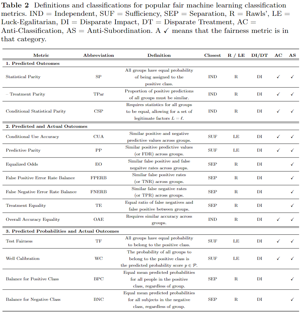
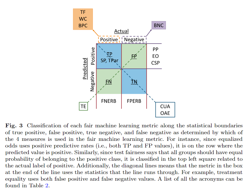
In this section I list several popular statistics-based fair machine learning metrics into categories based on several axes, including: what attributes of the machine learning system they use (e.g., the predicted outcomes, the predicted and actual outcomes, or the predicted probability and actual outcomes), which formal statistical criterion (independence, separation, or sufficiency) it aligns with as proposed in [3], which legal notion it can be tied to, as well as which philosophical ideal serves as its foundation (e.g., substantive (Rawls’) EOP or luck-egalitarian EOP) by using the classification procedure explained in [4,5]. Fig. 3 shows our classification of the metrics along the statistical lines of true positive, true negative, false positive, and false negative depending on what metrics the fairness method uses and Table 2 summarizes our main classification conclusions. Additionally, at the end of this section, we devote space to discussing individual fairness and the (apparent) differences between individual and group fair machine learning metrics. We additionally note that this section uses the following variables: $S=1$ is the marginalized or minority group, $S = 0$ is the non-marginalized or majority group, $\hat{Y}$ is the predicted value or class (i.e., label), and $Y$ is the true or actual label/class.

To provide a background for the following proofs, we state a relaxed, binary, version of the definitions for Rawls’ EOP and luck-egalitarian EOP for supervised learning proposed by Heidari et al 4:

Definition: Rawls’ and Luck-Egalitarian EOP for Supervised Learning]

Predictive model $h$ satisfies Rawlsian/Luck-Egalitarian EOP if for all $s\in S={0,1}$ and all $y, \hat{y} \in Y, \hat{Y} = {0,1} $:

$\text{Rawls': } F^h(U \leq u\mid S = 0 \cap Y = y) = F^h(U \leq u \mid S = 1 \cap Y = y)$

$\text{LE: } F^h(U \leq u\mid S = 0 \cap \hat{Y} = \hat{y}) = F^h(U \leq u \mid S = 1 \cap \hat{Y} = \hat{y})$

where $F^h(U \leq u)$ specifies the distribution of utility $U$ (i.e., the distribution of winning a social competition like being admitted to a university) across individuals under the predictive model $h$. I.e., it is the difference between the individual’s actual effort $A$ and their circumstance $D$, $U = A - D$. In this relaxed case, utility is the difference between the individual’s predicted and actual class.

Predicted Outcomes

The predicted outcomes family of fair machine learning metrics are the simplest, and most intuitive, notions of fairness. More explicitly, the predicted outcome class of metrics focuses on using the predicted outcome of various different demographic distributions of the data, and models only satisfy this definition if both the marginalized and non-marginalized groups have equal probability of being assigned to the positive predictive class [5]. Many different metrics fall into the predicted outcome category, such as statistical parity and conditional statistical parity. Additionally, each metric in this group satisfies Rawls’ definition of EOP as well as satisfies the statistical constraint of independence and the legal notions of anti-classification and anti-subordination. We also note that in the process of certifying and removing bias using fair machine learning metrics from this category, it is common to use the actual labels in place of the predicted labels (see Definition 1.1 of [6]). But, for simplicity, we present the fair machine learning metrics of this section using the predicted outcome only.

Statistical Parity

Statistical parity is also often called demographic parity, statistical fairness, equal acceptance rate, or benchmarking. As the name implies, it requires that there is an equal probability for both individuals in the marginalized and non-marginalized groups to be assigned to the positive class [7]. Notationally, statistical parity can be written as:

$P[\hat{Y} = 1 \mid S = 0] = P [\hat{Y} = 1 \mid S = 1]$

In [8], Heidari et al. map statistics-based fair machine learning metrics to equality of opportunity (EOP) models from political philosophy. In EOP an individual’s outcome is affected by their circumstance $c$ (all ‘irrelevant’ factors like race, gender, status, etc. that a person should not be held accountable for) and effort $e$ (those items which a person can morally be held accountable for). For any $c$ and $e$, a policy $\phi$ can be used to create a distribution of utility $U$ (e.g., the acceptance to a school, getting hired for a position, etc.) among the people with circumstance $c$ and effort $e$.

To map the notions of circumstance and effort to the proposed statistics-based fair machine learning notions, they treat the predictive model $h$ as policy $\phi$ and assume that a person’s features can be divided into those that are ‘irrelevant’ and those that they can be held accountable for (a.k.a, are effort-based). Additionally, they let the person’s irrelevant features be seen as their individual circumstance ( $\mathbf{z}$ for $c$ ), their effort-based utility as their effort ($d$ for $e$), and their utility be the difference between their actual-effort $a$ and effort-based utility $d$. The difference between $a$ and $d$ is much like the difference between $y$ and $\hat{y}$ in machine learning literature. In other words, $d$ is the utility a person should receive based on their accountable factors (i.e., the salary a person should receive based on their experience/education/etc.) while $a$ is the utility a person actually receives (i.e., the actual salary they are paid). Here, we recall the proof for statistical parity as Rawls’ EOP as presented in [8]

Proposition: Statistical Parity as Rawls’ EOP [8]

Consider the binary classification task where $Y, \hat{Y}={0,1}$. Suppose $U = A - D$, $A = \hat{Y}$, and $D = Y = 1$ (i.e., the effort-based utility of all individuals is assumed to be the same). Then, the conditions of Rawls’ EOP is equivalent to statistical parity when $\hat{Y} = 1$.

**Proof: ** Recall that Rawls’ EOP requires that $s\in S = {0,1}$ , $y \in Y= {0,1}$ , $u = a - d\in{-1, 0}$ :

$P[U\leq u \mid S = 0 \cap Y = y] = P [U \leq u \mid S = 1 \cap Y = y]$

Replacing $U$ with $(A - D)$, $D$ with 1, and $A$ with $\hat{Y}$ , the above is equivalent to:

$P[A - D \leq u \mid S = 0 \cap Y = 1] = P[A - D \leq u \mid S = 1 \cap Y = 1]$

$P[\hat{Y} - 1 \leq u \mid S = 0 \cap Y = 1] = P[\hat{Y} - 1 \leq u \mid S = 1 \cap Y = 1]$

$P[\hat{Y} \leq u + 1\mid S = 0] = P[\hat{Y} \leq u + 1 \mid S = 1]$

$P[\hat{Y} = \hat{y}\mid S = 0] = P[\hat{Y} = \hat{y} \mid S = 1]$

because of the facts that $u = \hat{y} - y$ and $y = 1$ produce the result $\hat{y} = u + 1$. This is equal to the definition for statistical parity when $\hat{Y} = 1$, therefore, the conditions of Rawls’ EOP is equivalent to statistical parity.

Treatment Parity

Instead of measuring the difference between the assignment rates, treatment parity looks at the ratio between the assignment rate. It is not a derivative of statistical parity as much as it is a different way of looking at it. The distinction between the forms of statistical parity and treatment parity was made to better connect with the legal term of disparate impact - as the treatment parity form was explicitly designed to be the mathematical counterpart to the legal notion [6, 9]. Mathematically, it is defined as:

$\frac{P[\hat{Y} = 1 \mid S = 0]}{P[\hat{Y} = 1 \mid S = 1]} \geq 1 - \epsilon$

where $\epsilon$ is the allowed slack of the metric and is usually set to $0.2$ to achieve the $80\%$ rule of disparate impact law. This equation says that the proportion of positive predictions for both the marginalized and non-marginalized groups must be similar (around threshold $1 - \epsilon$ ). Since it is essentially the same as statistical parity, it also aligns with Rawls’ EOP, independence, anti-classification, and anti-subordination.

Conditional Statistical Parity

Conditional statistical parity is an extension of statistical parity which allows a certain set of legitimate attributes to be factored into the outcome [10]. Factors are considered “legitimate” if they can be justified by ethics, by the law, or by a combination of both. This notion of fairness was first defined by Kamiran et al. in 2013 who wanted to quantify explainable and illegal discrimination in automated decision making where one or more attributes could contribute to the explanation [11]. Conditional statistical parity is satisfied if both marginalized and non-marginalized groups have an equal probability of being assigned to the positive predicted class when there is a set of legitimate factors that are being controlled for. Notationally, it can be written as:

$P[\hat{Y} = 1 \mid L_1 = a \cap L_2 = b \cap S = 0] = P[\hat{Y} = 1 \mid L_1 = a \cap L_2 = b \cap S = 1]$

where $L_1, L_2$ are legitimate features that are being conditioned on. For example, if the task was to predict if a certain person makes over $50,000 a year, then $L_1$ could represent work status and $L_2$ could be the individuals relationship status. Another, simplified way to write this can be seen as:

$P[\hat{Y} = 1 \mid L = \ell \cap S = 1] = P[\hat{Y} = 1 \mid L = \ell \cap S = 0]$

where $\ell\in L$ is the set of legitimate features being conditioned on.

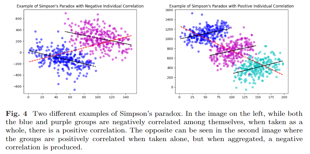
Furthermore, conditional statistical parity helps to overcome Simpson’s paradox as it incorporates extra conditioning information beyond the original class label. Simpson’s paradox says that if a correlation occurs in several different groups, it may disappear, or even reverse, when the groups are aggregated [12]. This event can be seen in Fig. 4.

Put mathematically, Simpson’s paradox can be written as:

$P[A \mid B \cap C] < P [A \mid B^c \cap C] \text{ and } P[A \mid B \cap C^c] < P [A \mid B^c \cap C^c]$

but

$P[A\mid B] > P[A\mid B^c]$

where $X^c$ denotes the complement of the variable. An analysis that does not consider all of the relevant statistics might suggest that unfairness and discrimination is at play, when in reality, the situation may be morally and legally acceptable if all of the information was known. As with the above two metrics, conditional statistical parity aligns with Rawls’ EOP, independence, anti-classification, and anti-subordination.

Predicted and Actual Outcomes

The predicted and actual outcome class of metrics uses both the model’s predictions as well as the true labels of the data. This class of fair machine learning metrics includes: predictive parity, false positive error rate balance, false negative error rate balance, equalized odds, conditional use accuracy, overall accuracy equality, and treatment equality.

Conditional Use Accuracy

Conditional use accuracy, also termed as predictive value parity, requires that positive and negative predicted values are similar across different groups [13]. Statistically, it aligns exactly with the requirement for sufficiency and therefore also aligns with anti-classification and anti-subordination [3]. Mathematically, it can be written as follows:

$P[Y = y \mid \hat{Y} = y \cap S = 0] = P[Y = y \mid \hat{Y} = y \cap S = 1] \;\; \text{ for } \;\; y\in\{0,1\}$

In [8], they provide a proof that conditional use accuracy falls into the luck-egalitarian EOP criterion and we recall their work below:

Proposition: Conditional Use Accuracy as Luck-Egalitarian EOP [8]

Consider the binary classification task where $y \in Y = {0,1}$ . Suppose that $U = A - D$, $A = Y$, and $D = \hat{Y}$ (i.e., the effort-based utility of an individual under model a $h$is assumed to be the same as their predicted label). Then the conditions of luck-egalitarian EOP are equivalent to those of conditional use accuracy (otherwise known as predictive value parity).

Proof: Recall that luck-egalitarian EOP requires that for $s\in S = {0,1}$, $\hat{y}\in\hat{Y}={0,1}$, and $u \in {-1, 1}$:

$P[U \leq u \mid \hat{Y}=\hat{y} \cap S = 0 ] = P[U \leq u \mid \hat{Y}=\hat{y} \cap S = 1 ]$

Replacing $U$ with $A - D$, $D$ with $\hat{Y}$, and $A$ with $Y$, we obtain the following:

$P[A - D \leq u \mid \hat{Y} = \hat{y} \cap S = 0 ] = P[A - D \leq u \mid \hat{Y}=\hat{y} \cap S = 1 ]$

$P[Y - \hat{Y} \leq u \mid \hat{Y} = \hat{y} \cap S = 0 ] = P[Y - \hat{Y} \leq u \mid \hat{Y}=\hat{y} \cap S = 1 ]$

$P[Y \leq u + \hat{y}\mid \hat{Y} = \hat{y} \cap S = 0 ] = P[Y \leq u + \hat{y}\mid \hat{Y}=\hat{y} \cap S = 1 ]$

$P[Y = y \mid \hat{Y} = \hat{y} \cap S = 0 ] = P[Y = y \mid \hat{Y}=\hat{y} \cap S = 1 ]$

since $u = a - d = y - \hat{y}$ produces the result that $y = u + \hat{y}$. The last line is then equal to the statement for conditional use accuracy when $y = \hat{y} = {0,1}$ .

Predictive Parity

Predictive parity, otherwise known by the name outcome test, is a fair machine learning metric that requires the positive predictive values to be similar across both marginalized and non-marginalized groups [14]. Mathematically, it can be seen as:

$P[Y=y \mid \hat{Y} = 1\cap S = 0] = P[Y=y\mid \hat{Y} = 1 \cap S = 1] \;\; \text{ for } \;\; y\in\{0,1\}$

since if a classifier has equal positive predictive values for both groups, it will also have equal false discovery rates. Since predictive parity is simply conditional use accuracy when $\hat{Y} = 1$, it falls into the same philosophical category as conditional use accuracy, which is luck-egalitarian EOP. Further, [3] states that predictive parity aligns with sufficiency. Since it aligns with sufficiency, it also aligns with anti-classification and anti-subordination.

Equalized Odds

The fair machine learning metric of equalized odds is also known as conditional procedure accuracy equality and disparate mistreatment. It requires that true and false positive rates are similar across different groups [15].

$P[\hat{Y} = 1 \mid Y = y \cap S = 0] = P[\hat{Y} = 1 \mid Y = y \cap S = 1] \;\; \text{ for } \;\; y\in\{0,1\}$

Equalized odds aligns with Rawls’ EOP and [8] provides a proof for this classification. Additionally, it aligns with separation and anti-subordination [3].

False Positive Error Rate Balance

False positive error rate balance, otherwise known as predictive equality, requires that false positive rates are similar across different groups [14]. It can be seen mathematically as:

$P[\hat{Y}=\hat{y} \mid Y = 0 \cap S = 0] = P[\hat{Y} = \hat{y} \mid Y = 0 \cap S = 1] \;\; \text{ for } \;\; \hat{y}\in\{0,1\}$

We note that if a classifier has equal false positive rates for both groups, it will also have equal true negative rates, hence why $\hat{y} \in {0,1}$. This fairness metric can be seen as a relaxed version of equalized odds that only requires equal false positive rates, and therefore it aligns with all the categories that equalized odds does, specifically: Rawls’ EOP, separation, and anti-subordination.

False Negative Error Rate Balance

False negative error rate balance, also called equal opportunity, is the direct opposite of the above fair machine learning metric of false positive error rate balance in that it requires false negative rates to be similar across different groups [14]. This metric can be written as:

$P[\hat{Y}=\hat{y} \mid Y = 1 \cap S = 0] = P[\hat{Y} = \hat{y} \mid Y = 1 \cap S = 1] \;\; \text{ for } \;\; \hat{y}\in\{0,1\}$

and we note that a classifier that has equal false negative rates across the two groups will also have equal true positive rates. This fair machine learning metric can also be seen as a relaxed version of equalized odds that only requires equal false negative error rates, and therefore, aligns with all the same categories.

Overall Accuracy Equality

As the name implies, overall accuracy equality requires similar prediction accuracy across different groups. In this case, we are assuming that obtaining a true negative is as desirable as obtaining a true positive [16]. According to [3], it matches with the statistical measure of independence, meaning that it also aligns with anti-classification and anti-subordination. Mathematically, it can be written as:

$P[\hat{Y}=y \mid Y = y \cap S = 0] = P[\hat{Y} = y\mid Y = y \cap S = 1] \;\; \text{ for } \;\; y, \hat{y} \in \{0,1\}$

Overall accuracy equality is the third fair machine learning metric that Heidari et al. prove belongs to the Rawls’ EOP category of fair machine learning metrics [8].

Treatment Equality

Treatment equality analyzes fairness by looking at how many errors were obtained rather than through the lens of accuracy. It requires an equal ratio of false negative and false positive values for all groups [16]. Further, it agrees exactly with the statistical measure of separation [3], and the legal notion of anti-subordination.

$\frac{FN_{S = 0}}{FP_{S = 0}} = \frac{FN_{S = 1}}{FP_{S = 1}}$

Treatment equality can be considered as the ratio of false positive error rate balance and false negative error rate balance. Since both of these metrics fall into the Rawls’ EOP category, treatment equality does as well.

Predicted Probabilities and Actual Outcomes

The predicted probability and actual outcome category of fair machine learning metrics is similar to the above category of metrics that use the predicted and actual outcomes. But, instead of using the predictions themselves, this category uses the probability of being predicted to a certain class. This category of metrics includes: test fairness, well calibration, balance for the positive class, and balance for the negative class. The first two metrics fall in line with the statistical measure of sufficiency and legal notions of both anti-classification and anti-subordination, while the last two align with separation and anti-subordination.

Test Fairness

Test fairness, which falls under the luck-egalitarian EOP category, is satisfied if, for any predicted probability score $p \in \mathcal{P}$, subjects in both the marginalized and non-marginalized groups have equal probability of actually belonging to the positive class. Test fairness has also been referenced by the terms calibration, equal calibration, and matching conditional frequencies [14]. Mathematically, it can be written as follows:

$P[Y = 1 \mid \mathcal{P} = p \cap S = 0] = P[Y = 1 \mid \mathcal{P} = p \cap S = 1]$

Well Calibration

Well calibration is very similar to the metric of test fairness, but it additionally requires that for any predicted probability score $p \in \mathcal{P}$, not only should the majority and minority classes have equal probability of belonging to the positive class, but this probability should be $p$ [17].

$P[Y=1\mid \mathcal{P}=p \cap S = 0] = P[Y=1\mid \mathcal{P}=p \cap S = 1] = p$

Since well calibration is an extension of test fairness, it also falls under the classifications of luck-egalitarian EOP, sufficiency, anti-classification, and anti-subordination.

Balance for the Positive Class

As the name suggests, the balance for the positive class metric requires that individuals who experience a positive outcome, regardless of which group they belong to, should have an equal mean predicted probability of being in the positive class [17]. It can be seen as being similar to the metric of equal opportunity, which says that a classifier should give equivalent treatment to all groups.

$\mathbb{E}[\mathcal{P} \mid Y = 1 \cap S = 0] =\mathbb{E}[\mathcal{P} \mid Y = 1 \cap S = 1]$

Like false positive error rate balance, the balance for the positive class metric can be seen as a derivative of the equalized odds metric when $Y = 1$. Additionally, instead of taking into account the predicted label $\hat{y} \in \hat{Y}$, it concerns itself with the predicted probability $\mathcal{P}$. Since equalized odds falls into Rawls’ EOP category of metrics, the balance for the positive class metric does as well. Similarly, balance for the positive class also aligns with separation and anti-subordination.

Balance for the Negative Class

The metric of balance for the negative class is opposite of the balance for the positive class metric. Instead of requiring balance in the predictive mean of the positive class, it requires balance in the predicted mean of the negative class [17]. It is similar to the measure of false positive error rate balance.

$\mathbb{E}[\mathcal{P} \mid Y = 0 \cap S = 0] =\mathbb{E}[\mathcal{P} \mid Y = 0 \cap S = 1]$

Same as the argument for balance for the positive class, the balance for the negative class metric is a derivative of equalized odds when $Y = 0$ and we approximate $\hat{y} \in \hat{Y}$ with probability score $\mathcal{P}$. Therefore, the balance for the negative class metric falls under all the same categorization as equalized odds (as well as balance for the positive class) does.